5.1 Linear algebra: vectors

For our purposes, a vector is a collection of real numbers in a one- dimensional array.We usually think of the array as being arranged in a column and write complete course in linear algebra and introduce only the functional techniques necessary to solve the problems at hand.

$x=x_1{x}_2{x}_3|x_n$ .

Notice that we indicate a vector with boldface and the constituent elements with subscripts. A real number by itself is called a scalar , in distinction from a vector or a matrix. We say that $x$ is an n-vector, meaning that $x$ has $n$ elements. To indicate that $x_1$ is a real number, we write

meaning that $x_1$ is contained in $R$ , the set of real numbers. To indicate that $x$ is a vector of $n$ real numbers, we write

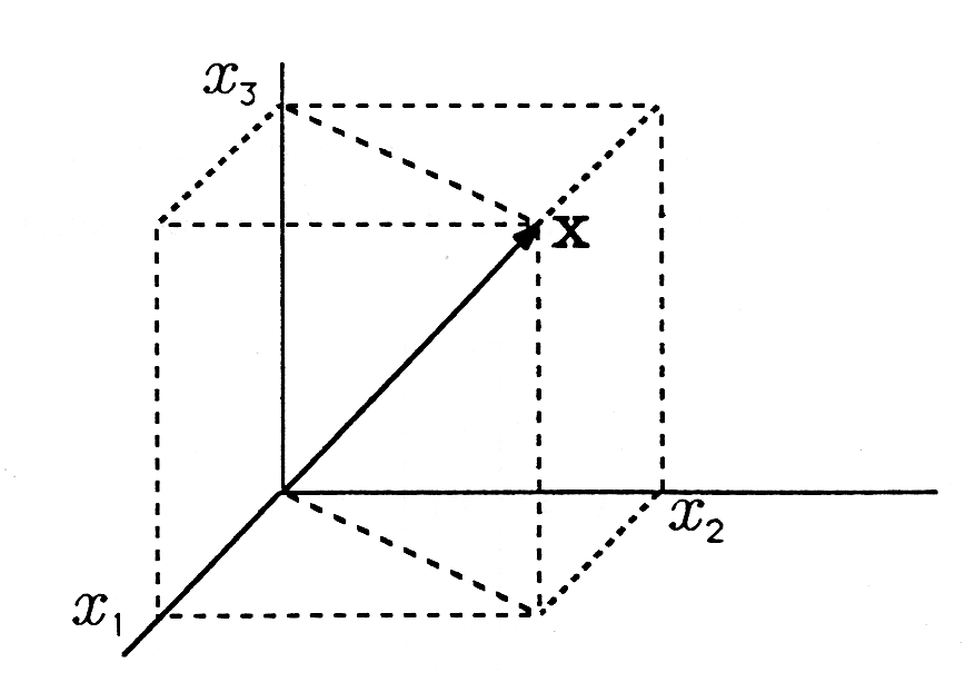
meaning that $x$ is contained in $R^n$ , the set of real n-tuples. Geometrically, $R^n$ is n-dimensional space, and the notation $x\in R^n$ means that $x$ is a point in that space, specified by the $n$ coordinates $x_1,x_2,...,x_n$ . [link] shows a vector in $R^3$ , drawn as an arrow from the origin to the point $x$ . Our geometric intuition begins to fail above three dimensions, but the linearalgebra is completely general.

We sometimes find it useful to sketch vectors with more than three dimensions in the same way as the three-dimensional vector of [link] . We then consider each axis to represent more than one dimension, a hyperplane, inour n-dimensional space. We cannot show all the details of what is happening in n-space on a three-dimensional figure, but we can often show importantfeatures and gain geometrical insight.

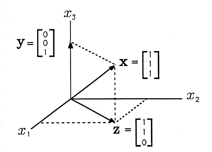
Vector Addition. Vectors with the same number of elements can be added and subtracted in a very natural way:

The difference between the vector $x=111$ and the vector $y=001$ is the vector $z=x-y=110$ . These vectors are illustrated in [link] . You can see that this result is consistent with the definition of vector subtraction in [link] . You can also picture the subtraction in [link] by mentally reversing the direction of vector $y$ to get $-y$ and then adding it to $x$ by sliding it to the position where its tail coincides with the head of vector $x$ . (The head is the end with the arrow.) When you slide a vector to a new position for adding to another vector, you must not changeits length or direction.

Scalar Product. Several different kinds of vector multiplication are defined.We begin with the scalar product . Scalar multiplication is defined for scalar $a$ and vector $x$ as The division of two vectors is undefined, although three different “divisions” are defined in MATLAB.

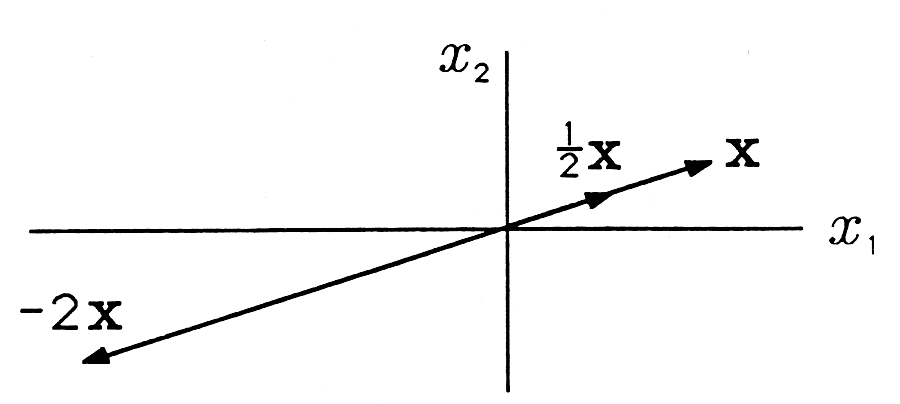
If $\left|a\right|<1$ , then the vector $ax$ is "shorter" than the vector x ; if $\left|a\right|>1$ , then the vector $ax$ is ‚"longer" than x . This is illustrated for a 2-vector in [link] .