3.7 Filters

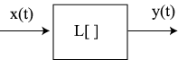
Filters are devices which are commonly found in electronic gadgets. When you adjust the bass (low frequency) or treble (high frequency) settings on your MP3 player, you are adjusting the characteristics of a filter. A more technical name for a filter is a linear system . A filter is represented by a box having a single input (usually $x\left(t\right)$ ) and a single output (say, $y\left(t\right)$ ) as seen in [link] .

We can denote the operation the filter has on the input using the following notation:

The types of filters we will consider in this book are linear and time-invariant . A filter is time-invariant if given that $y\left(t\right)=L\left[x,\left(,t,\right)\right]$ , then $y(t-\tau )=L\left[x,(,t,-,\tau ,)\right]$ . In other words, if the input to the filter is delayed by $\tau$ , then the output is also delayed by $\tau$ . A filter is linear if given that $y_1\left(t\right)=L\left[x_1,\left(t\right)\right]$ and $y_2\left(t\right)=L\left[x_2,\left(t\right)\right]$ then

Equation [link] is often referred to as the superposition principle . We can use linearity and time invariance to derive the mathematical operation which the filter performs on the input, $x\left(t\right)$ . To do this we begin with the assumption that

The signal $h\left(t\right)$ is called the impulse response of the filter. From time invariance, we have

Now we can use linearity to find the filter output when the input is $x\left(\tau \right)\delta (t-\tau )$ , where $x\left(\tau \right)$ is a constant

We can extend the linearity property further by noting that

where we can assume that the constants ${\tau }_n$ are ordered so that ${\tau }_i<{\tau }_k,i<k$ and ${\Delta }_n\equiv {\tau }_n-{\tau }_{n-1}$ . In [link] , we are simply multiplying each $\delta (t-{\tau }_n)$ by the constant $x\left({\tau }_n\right){\Delta }_n$ , so once again linearity should prevail. Now if we take the limit ${\Delta }_n\to 0$ , we obtain

Using the sifting property of the unit impulse in the right side of [link] gives

So it follows that the filter performs the following operation on the input, $x\left(t\right)$ :

The integral in [link] is called the convolution integral . A change of variables can be used to show that

which means that the order in which two signals are convolved is unimportant. A short-hand notation for convolution is