

| << Chapter < Page | Chapter >> Page > |
The Butterworth filter does not give a sufficiently good approximation across the complete passband in many cases. TheTaylor's series approximation is often not suited to the way specifications are given for filters. An alternate error measure isthe maximum of the absolute value of the difference between the actual filter response and the ideal. This is considered over thetotal passband. This is the Chebyshev error measure and was defined and applied to the FIR filter design problem. For the IIR filter,the Chebyshev error is minimized over the passband and a Taylor's series approximation at is used to determine the stopband performance. This mixture of methods in the IIR case iscalled the Chebyshev filter, and simple design formulas result, just as for the Butterworth filter.
The design of Chebyshev filters is particularly interesting, because the results of a very elegant theory insure thatconstructing a frequency-response function with the proper form of equal ripple in the error will result in a minimum Chebyshev errorwithout explicitly minimizing anything. This allows a straightforward set of design formulas to be derived which can beviewed as a generalization of the Butterworth formulas [link] , [link] .
The form for the magnitude squared of the frequency-response function for the Chebyshev filter is
where is an Nth-order Chebyshev polynomial and is a parameter that controls the ripple size. This polynomial in has very special characteristics that result in the optimality of the response function [link] .
The Chebyshev polynomial is a powerful function in approximation theory. Although the function is a polynomial, it isbest defined and developed in terms of trigonometric functions by [link] , [link] , [link] , [link] .
where is an Nth-order, real-valued function of the real variable . The development is made clearer by introducing an intermediate complex variable .
where
Although this definition of may not at first appear to result in a polynomial, the following recursive relation derivedfrom [link] shows that it is a polynomial.
From [link] , it is clear that and , and from [link] , it follows that
etc.
Other relations useful for developing these polynomials are
where M and N are coprime.
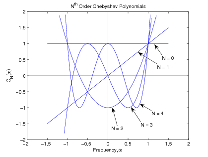
These are remarkable functions [link] . They oscillate between +1 and -1 for and go monotonically to +/- infinity outside that domain. All of their zeros are real and fall in the domain of , i.e., is an equal ripple approximation to zero over the range of from -1 to +1. In addition, the values for where reaches its local maxima and minima and is zero are easily calculated from [link] and [link] . For , a plot of can be made using the concept of Lissajous figures. Example plots for , , , , and are shown in [link] .
The filter frequency-response function for is given in [link] showing the passband ripple in terms of the parameter .
Notification Switch
Would you like to follow the 'Digital signal processing and digital filter design (draft)' conversation and receive update notifications?

|
|

|
|

|
|

|
|

|
|

|
|

|
|

|
|

|
|

|