3.2 Calculus of variations

The calculus of variations refers to a generic class of optimization problems that can be written in terms of

where $J\left(x\right):C[t_1,t_2]\to R$ is a function that can be written as

where $\dot{x}\left(t\right)=\frac{dx\left(t\right)}{dt}$ . The function $f$ must meet the following conditions:

• $f(x\left(t\right),\dot{x}\left(t\right),t)$ is continuous on $x\left(t\right)$ , $\dot{x}\left(t\right)$ , and $t$ as individual inputs,
• $f(x\left(t\right),\dot{x}\left(t\right),t)$ has continuous partial derivatives with respect to $x\left(t\right)$ and $\dot{x}\left(t\right)$ , written as
  $$\begin{array}{cc}\hfill f_x(x\left(t\right),\dot{x}\left(t\right),t)& =\frac{\partial }{\partial x}{f}_x(x\left(t\right),\dot{x}\left(t\right),t),\hfill \\ \hfill f_{\dot{x}}(x\left(t\right),\dot{x}\left(t\right),t)& =\frac{\partial }{\partial \dot{x}}{f}_x(x\left(t\right),\dot{x}\left(t\right),t).\hfill \end{array}$$

Consider the set of admissible functions $x\in C[t_1,t_2]$ . One can pick any particular admissible function $x$ and then define the rest of the set in terms of $x+h$ , where $h\left(t_1\right)=h\left(t_2\right)=0$ . Therefore, at an optimum $x$ , we require the directional derivative in the feasible directions h to be zero valued, i.e., $\partial J(x;h)=0$ for all feasible directions $h$ . Now recall that since $J\left(x\right)$ is scalar-valued, we have

We use the following fact:

Fact 1 For any function $g(x,y,z)$ , we have that

Therefore,

where we drop the dependence of the functions for brevity (i.e., $x\left(t\right)$ is written $x$ ). Using integration by parts ( $u=f_{\dot{x}}(x+\alpha x,\dot{x}+\alpha \dot{h},t)$ , $dv=\dot{h}dt$ ), we get

since $h\left(t_1\right)=h\left(t_2\right)=0$ , we have that

It follows that for $\partial J(x;h)=0$ for all feasible directions $\alpha$ , we must have

which provides the following condition on the solution $x\left(t\right)$ of the problem [link] :

This condition is known as the Euler-Lagrange equation.

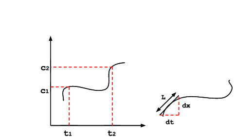
Example 1 Looking for a function $x\left(t\right)\in C[t_1,t_2]$ that minimizes the length of the path (curve) between the points $(t_1,c_1)$ and $(t_2,c_2)$ , as shown in [link] .

In this case, we can consider increments of the curve's length $l$ in terms of differences of the input $dt$ and the output $dx$ :

and by integrating both sides we get that

where we have written $f(x,\dot{x},t)=\sqrt{1+{\dot{x}}^2}$ , and the problem has set the boundary conditions $x\left(t_1\right)=c_1$ , $x\left(t_2\right)=c_2$ . Thus, we have a calculus of variations problem.

To obtain the solution to this problem, we set up the Euler-Lagrange equation:

in words, $f_{\dot{x}}(x,\dot{x},t)$ must be a constant as a function of $t$ , which implies that $\dot{x}\left(t\right)$ must be a constant function of $t$ ; such a function with constant first derivative is a straight line. Therefore, the shortest path between the two aforementioned points is obtained by the straight line that connects them.

Example 2 Consider a retirement plan with the following constraints:

• Your current capital is $S$ dollars, and ideally by the end of your life you will have spent it all; that is, if $x\left(t\right)$ is your capital at time $t$ , then $x\left(0\right)=S$ and $x\left(T\right)=0$ .
• Your expense rate is given by the function $r\left(t\right)$ , and spending $r$ dollars gives you a quantifiable amount of enjoyment $u\left[r\right(t\left)\right]$ .

The goal of the planning is to maximize your total enjoyment:

where the exponential weights enjoyment to specify that enjoyment decreases with age. The change in your capital is given by its derivative, which must account for your expense rate and the return on investment:

where $\alpha >1$ . The problem is thus to maximize the function of your capital function

which together with the initial constraints gives us a calculus of variation problem. Thus, once again, we set up the Euler-Lagrange equation: if we denote $u^{\text{'}}\left[r\right]=\frac{d}{dr}u\left[r\right]$ , then

So we obtain

Now we can switch back to the rate of expense $r\left(t\right)=\alpha x\left(t\right)-\dot{x}\left(t\right)$ to get

which is a differential equation. The solution for $u^{\text{'}}\left[r\left(t\right)\right]$ is therefore given by

To move forward, we need to select a candidate form for the utility function $u$ . Our goals for this function is to showcase a diminishing marginal enjoyment as one spends increasing amounts of money (i.e., $u^{\text{'}}\left[m\right]\to 0$ as $m\to \infty$ ) and a sense of significantly increasing enjoyment as the amount of money spent is small but increasing (i.e., $u^{\text{'}}\left(0\right)=\infty$ ). A candidate function that obeys these two conditions is $u\left[m\right]=2m^{1/2}$ , which provides $u^{\text{'}}\left[m\right]=m^{-1/2}$ ; replacing in [link] , we get that the rate of expense must obey

Connecting back to the capital function, we get that

which is another differential equation. The solution to this equation is

In this equation we can replace $x\left(0\right)=S$ ; assuming $\alpha >\beta >\alpha /2$ , we can find $r\left(0\right)$ by setting $T=0$ above; since $x\left(T\right)=0$ , we get

Therefore, the final solution to the problem is