

| << Chapter < Page | Chapter >> Page > |
In the previous set of notes, we talked about the EM algorithm as applied to fitting a mixture of Gaussians. In this set of notes,we give a broader view of the EM algorithm, and show how it can be applied to a large family of estimation problemswith latent variables. We begin our discussion with a very useful result called Jensen's inequality
Let be a function whose domain is the set of real numbers. Recall that is a convex function if (for all ). In the case of taking vector-valued inputs, this is generalized to the condition that its hessian is positive semi-definite ( ). If for all , then we say is strictly convex (in the vector-valued case, the corresponding statement is that must be positive definite, written ). Jensen's inequality can then be stated as follows:
Theorem. Let be a convex function, and let be a random variable. Then:
Moreover, if is strictly convex, then holds true if and only if with probability 1 (i.e., if is a constant).
Recall our convention of occasionally dropping the parentheses when writing expectations, so in the theorem above, .
For an interpretation of the theorem, consider the figure below.
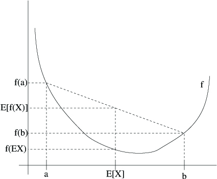
Here, is a convex function shown by the solid line. Also, is a random variable that has a 0.5 chance of taking the value , and a 0.5 chance of taking the value (indicated on the -axis). Thus, the expected value of is given by the midpoint between and .
We also see the values , and indicated on the -axis. Moreover, the value is now the midpoint on the -axis between and . From our example, we see that because is convex, it must be the case that .
Incidentally, quite a lot of people have trouble remembering which way the inequality goes, and remembering a picture like this isa good way to quickly figure out the answer.
Remark. Recall that is [strictly] concave if and only if is [strictly]convex (i.e., or ). Jensen's inequality also holds for concave functions , but with the direction of all the inequalities reversed ( , etc.).
Suppose we have an estimation problem in which we have a training set consisting of independent examples. We wish to fit the parameters of a model to the data, where the likelihood is given by
But, explicitly finding the maximum likelihood estimates of the parameters may be hard. Here, the 's are the latent random variables; and it is often the case that if the 's were observed, then maximum likelihood estimation would be easy.
In such a setting, the EM algorithm gives an efficient method for maximum likelihood estimation. Maximizing explicitly might be difficult, and our strategy will be to instead repeatedlyconstruct a lower-bound on (E-step), and then optimize that lower-bound (M-step).
For each , let be some distribution over the 's ( , ). Consider the following: If were continuous, then would be a density, and the summations over in our discussion are replaced with integrals over .
Notification Switch
Would you like to follow the 'Machine learning' conversation and receive update notifications?

|
|

|
|

|
|

|
|

|
|
|
|
|

|
|

|
|
|
|
|

|