2.6 Matrix representations of linear operators

Linear operators involving finite-dimensional spaces can be represented in terms of matrices. Assume that $X$ and $Y$ are finite-dimensional spaces and $A\in B(X,Y)$ . Let I $\left\{e_i\right\}$ be a orthonormal basis for $X$ so that for all $x\in X$ we have $x={\sum }_i⟨x,e_i⟩e_i$ , giving $x$ the unique set of coefficients $a_i=⟨x,e_i⟩$ . Similarly, let $\left\{{\tilde{e}}_i\right\}$ be an orthonormal basis for $Y$ so that for $y\in Y$ we have $y={\sum }_i⟨y,{\tilde{e}}_i⟩{\tilde{e}}_i$ , giving $y$ the unique set of coefficients $b_i=⟨y,{\tilde{e}}_i⟩$ . We will now show that the map $x\to y=A\left(x\right)$ can be represented in terms of their coefficient vectors as $a\to b=\tilde{A}a$ , where $\tilde{A}$ is a matrix.

Recall that ${\psi }_i=A{e}_i\in Y$ , so it can be written as ${\psi }_i={\sum }_j⟨{\psi }_i,{\tilde{e}}_j⟩{\tilde{e}}_j$ . Therefore,

Due to the uniqueness of coefficients for $y$ in $\left\{{\tilde{e}}_j\right\}$ , we have that for each $j$ ,

So we have found a matrix $\tilde{A}$ with entries ${\tilde{A}}_{j,i}=⟨{\psi }_i,{\tilde{e}}_j⟩$ that provides $\tilde{A}a=b$ . Note that the matrix will be of size $\dim \left(Y\right)\times \dim \left(X\right)$ .

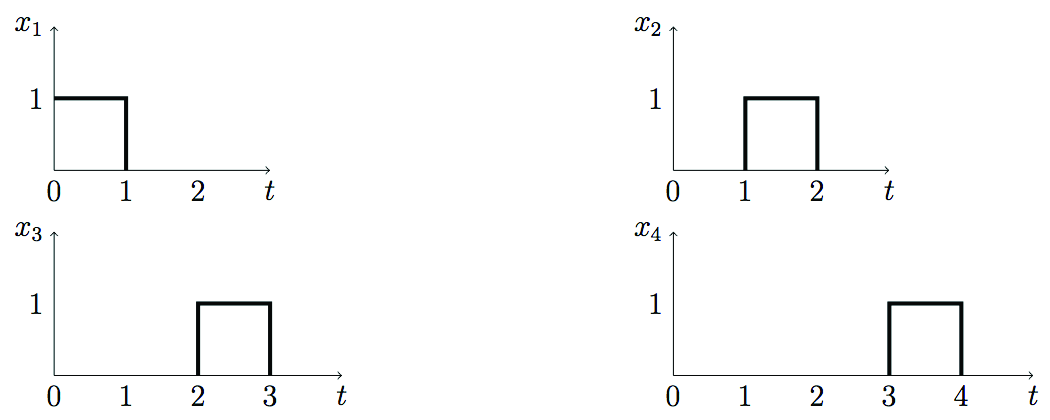
Example 1 Consider the space $X\subseteq L_2[0,1]$ defined by $X=\mathrm{span}\left(\{x_1,x_2,x_3,x_4\}\right)$ , given below:

and the space $Y\subseteq L_2[0,4]$ given by $Y=\mathrm{span}\left(\{y_1,y_2\}\right)$ , where $y_1\left(t\right)=\sqrt{2}cos\left(2\pi t\right)$ and $y_2\left(t\right)=\sqrt{2}cos\left(4\pi t\right)$ . We define an operator $A:X\to Y$ as

It is easy to see that an orthonormal basis for $X$ is given by the functions $e_i\left(t\right)=x_i\left(t\right)$ . One can also show that an orthonormal basis for $Y$ is given by the functions ${\tilde{e}}_1\left(t\right)=\frac{1}{\sqrt{2}}cos\left(2\pi t\right)$ and ${\tilde{e}}_2\left(t\right)=\frac{1}{\sqrt{2}}cos\left(4\pi t\right)$ . For this choice of orthonormal bases for $X$ and $Y$ , the transformed basis elements from $X$ are given by

It is then easy to check that the entries of the matrix are given by

Thus, the matrix representation for the operator $A$ using these orthonormal bases is given by