2.2 Panel data models  (Page 7/10)

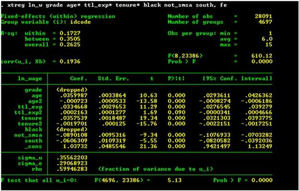
The estimates of the parameter values for the fixed-effects model are very similar to those found for the random-effects model with the exception for the parameters associated with not living in an SMSA ( not_smsa ) and with living in the South ( south ). The random-effects model suggests that the wage level for someone living outside of a SMSA is 87.6 percent of the wage level of someone living in an SMSA; in the fixed-effects model, the wage level outside the SMSA is estimated to be 91.5 percent of the wage level of a woman living in a SMSA. The random-effects model estimates wages in the South are 91.6 percent the level of wages outside the South; the fixed-effects model fixes this wage premium at 91.6 percent.

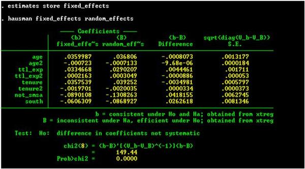
The final issue we discuss in this example is the Hausman specification test. If the model is correctly specified and if ν _i is uncorrelated with the explanatory variables, then the parameter estimates in the two models should not be statistically different. As shown in Figure 8, we first must same the results of the fixed-effects estimation using the command estimates store fixed_effects . The null hypothesis is that the the difference in that parameter estimates is not systematic. The appropriate test statistic is the χ ² (8), where the degrees of freedom are equal to the number of parameters in the model (8). The chi-squared statistic of 149.44 is greater than the critical value and we must reject the null hypothesis. The Stata offers this interpretation of this result:

What does this mean? We have an unpleasant choice: we can admit that our model is misspecified—that we have not parameterized it correctly—or we can hold to our specification

being correct, in which case the observed differences must be due to the zero-correlation of and the assumption. [StataCorp: 202]

Exercises

where:

y _it = natural logarithm of individual i ’s wage rate in year t ,

h _it = natural logarithm of total number of hours worked by individual i in year t ,

Age _it = age of individual i in year t ,

NC _it = number of children of individual i in year t , and

HI _it = an dummy variable equal to 1 if individual i in year t has bad health and 0 otherwise.

The data are from Ziliak, James P. (1997) “Efficient Estimation with Panel Data When Instruments Are Predetermined: An Empirical Comparison of Moment-Condition Estimators,” Journal of Business&Economic Statistics 15 (4): 419-431. Ziliak (p. 423) describes his data as follows:

The data used to estimate the life-cycle labor-supply parameters come from Waves XII-XXI (calendar years 1978-1987) of the PSID. The sample is selected on many dimensions and is similar to other research studying life-cycle models of labor supply. The sample is restricted to continuously married, continuously working, prime-age men aged 22-51 in 1978 from the Survey Research Center random subsample of the PSID. In addition the individual must either be paid an hourly wage rate or must be salaried, and he cannot be a piece-rate worker or self-employed. This selection process resulted in a balanced panel of 532 men over 10 years or 5,320 observations. The real wage rate, w it ,. is the hourly wage reported by the panel participant rather than the average wage (annual earnings over annual hours) to minimize division bias (Borjas 1981).