2.10 Machine learning lecture 10 course notes

Principal components analysis

In our discussion of factor analysis, we gave a way to model data $x\in {\mathbb{R}}^n$ as “approximately” lying in some $k$ -dimension subspace, where $k\ll n$ . Specifically, we imagined that each point $x^{\left(i\right)}$ was created by first generating some $z^{\left(i\right)}$ lying in the $k$ -dimension affine space $\{\Lambda z+\mu ;z\in {\mathbb{R}}^k\}$ , and then adding $\Psi$ -covariance noise. Factor analysis is based on a probabilistic model, and parameter estimationused the iterative EM algorithm.

In this set of notes, we will develop a method, Principal Components Analysis (PCA), that also tries to identify the subspace in which the data approximately lies.However, PCA will do so more directly, and will require only an eigenvector calculation (easily done with the eig function in Matlab), and does not need to resort to EM.

Suppose we are given a dataset $\{x^{\left(i\right)};i=1,...,m\}$ of attributes of $m$ different types of automobiles, such as their maximum speed, turn radius, and so on. Let $x^{\left(i\right)}\in {\mathbb{R}}^n$ for each $i$ ( $n\ll m$ ). But unknown to us, two different attributes—some $x_i$ and $x_j$ —respectively give a car's maximum speed measured in miles per hour, and the maximum speed measured in kilometers per hour.These two attributes are therefore almost linearly dependent, up to only small differences introduced by rounding off to the nearest mph or kph. Thus, the data really lies approximatelyon an $n-1$ dimensional subspace. How can we automatically detect, and perhaps remove, this redundancy?

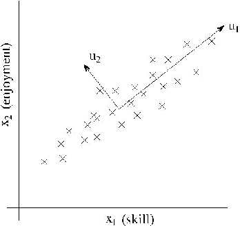
For a less contrived example, consider a dataset resulting from a survey of pilots for radio-controlled helicopters,where $x_1^{\left(i\right)}$ is a measure of the piloting skill of pilot $i$ , and $x_2^{\left(i\right)}$ captures how much he/she enjoys flying. Because RC helicopters are very difficult to fly,only the most committed students, ones that truly enjoy flying, become good pilots. So, the two attributes $x_1$ and $x_2$ are strongly correlated. Indeed, we might posit that that the data actually likes along some diagonalaxis (the $u_1$ direction) capturing the intrinsic piloting “karma” of a person, with only a small amount of noise lying off this axis. (See figure.) How can we automatically compute this $u_1$ direction?

We will shortly develop the PCA algorithm. But prior to running PCA per se, typically we first pre-processthe data to normalize its mean and variance, as follows:

1. Let $\mu =\frac{1}{m}{\sum }_{i=1}^m{x}^{\left(i\right)}$ .
2. Replace each $x^{\left(i\right)}$ with $x^{\left(i\right)}-\mu$ .
3. Let ${\sigma }_j^2=\frac{1}{m}{\sum }_i{\left(x_j^{\left(i\right)}\right)}^2$
4. Replace each $x_j^{\left(i\right)}$ with $x_j^{\left(i\right)}/{\sigma }_j$ .

Steps (1-2) zero out the mean of the data, and may be omitted for data known to have zero mean (for instance, time series corresponding to speech or other acoustic signals).Steps (3-4) rescale each coordinate to have unit variance, which ensures that different attributesare all treated on the same “scale.” For instance, if $x_1$ was cars' maximum speed in mph (taking values in the high tens or low hundreds) and $x_2$ were the number of seats (taking values around 2-4), then this renormalization rescales the different attributes to make themmore comparable. Steps (3-4) may be omitted if we had apriori knowledge that the different attributes are all on the same scale. One example of this is if each data point represented agrayscale image, and each $x_j^{\left(i\right)}$ took a value in $\{0,1,...,255\}$ corresponding to the intensity value of pixel $j$ in image $i$ .