11.2 Test of a single variance

Thus far our interest has been exclusively on the population parameter μ or it's counterpart in the binomial, p. Surely the mean of a population is the most critical piece of information to have, but in some cases we are interested in the variability of the outcomes of some distribution. In almost all production processes quality is measured not only by how closely the machine matches the target, but also the variability of the process. If one were filling bags with potato chips not only would there be interest in the average weight of the bag, but also how much variation there was in the weights. No one wants to be assured that the average weight is accurate when their bag has no chips. Electricity voltage may meet some average level, but great variability, spikes, can cause serious damage to electrical machines, especially computers. I would not only like to have a high mean grade in my classes, but also low variation about this mean. In short, statistical tests concerning the variance of a distribution have great value and many applications.

A test of a single variance assumes that the underlying distribution is normal . The null and alternative hypotheses are stated in terms of the population variance . The test statistic is:

where:

• n = the total number of data
• s ² = sample variance
• ${\sigma }_0^2$ = hypothesized value of the population variance
• $H_0:{\sigma }^2={\sigma }_0^2$
• $H_a:{\sigma }^2\ne {\sigma }_0^2$

You may think of s as the random variable in this test. The number of degrees of freedom is df = n - 1. A test of a single variance may be right-tailed, left-tailed, or two-tailed. [link] will show you how to set up the null and alternative hypotheses. The null and alternative hypotheses contain statements about the population variance.

With individual lines at its various windows, a post office finds that the standard deviation for waiting times for customers on Friday afternoon is 7.2 minutes. The post office experiments with a single, main waiting line and finds that for a random sample of 25 customers, the waiting times for customers have a standard deviation of 3.5 minutes.

With a significance level of 5%, test the claim that a single line causes lower variation among waiting times (shorter waiting times) for customers .

Since the claim is that a single line causes less variation, this is a test of a single variance. The parameter is the population variance, σ ² .

Random Variable: The sample standard deviation, s , is the random variable. Let s = standard deviation for the waiting times.

• H ₀ : σ ² = 7.2 ²
• H _a : σ ² <7.2 ²

The word "less" tells you this is a left-tailed test.

Distribution for the test: ${\chi }_{24}^2$ , where:

• n = the number of customers sampled
• df = n – 1 = 25 – 1 = 24

Calculate the test statistic:

${\chi }_c^2=\frac{(n-1)s^2}{{\sigma }^2}=\frac{(25-1){(3.5)}^2}{{7.2}^2}=5.67$

where n = 25, s = 3.5, and σ = 7.2.

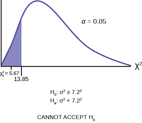
The graph of the Chi-square shows the distribution and marks the critical value with 24 degrees of freedom at 95% level of confidence, α = 0.05, 13.85. The graph also marks the calculated χ ² test statistic of 5.67. Comparing the test statistic with the critical value, as we have done with all other hypothesis tests, we reach the conclusion

Make a decision: Because the calculated test statistic is in the tail we cannot accept H ₀ . This means that you reject σ ² ≥ 7.2 ² . In other words, you do not think the variation in waiting times is 7.2 minutes or more; you think the variation in waiting times is less.

Conclusion: At a 5% level of significance, from the data, there is sufficient evidence to conclude that a single line causes a lower variation among the waiting times or with a single line, the customer waiting times vary less than 7.2 minutes.