10.1 Sspd-experiment number 2

Experiement -2

2.1. Aim

-To study the time domain and frequency domain response of RC circuit which is a first order system .

[The number of independent energy storage elements decide the order of the system. In a parallel or series LC resonance circuit the order is two. The order of a system gives the number of natural frequencies of the system. In first order system there is one natural frequency. This natural frequency decides rise-time/fall-time or the sag transients in TIME DOMAIN RESPONSE while it decides the cut-off frequency/-3dB frequency/0.707 frequency/half power frequency/corner frequency in Frequency Domain Response ]

2.2. Apparatus

- digital storage oscilloscope, breadboard, function generator.

2.3 Theory

–

1. The steady state sinusoidal response of the system under consideration is the Frequency Domain Response of the system.

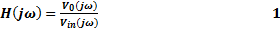
Transfer Function of a system = H(jω) = V _out (jω)/ V _in (jω).

This has a magnitude as well as a phase. The plot of the magnitude of H(jω) with respect to frequency is the Magnitude Frequency Response and Phase vs Frequency is Phase Frequency Response.

1. The time domain response is the square wave response of the system

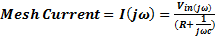
2.4. High pass RC circuit (as shown in Figure 1.a.)

The reactance of the series capacitance is given as

With increase in frequency, the reactance of the series capacitor decreases and therefore the transmission increases with frequency. At very high frequency the capacitive reactance become negligible so the output becomes almost equal to the input and transmission becomes 100%. Since the circuit attenuates the low frequency signals and allows transmission of high frequency signals with little or no attenuation, it is called high pass circuit. This circuit is widely employed as a coupling circuit in RC-coupled Amplifier. This helps isolate the Q-point of the Amplifier by the loading effect of the Source and the Load of the Amplifier.

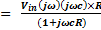
The voltage transfer function referring to Figure 1.a.

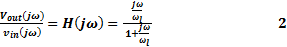
Equation 4 indicates that at low frequency the magnitude of the transfer function increases at +20dB per decade as shown in Figure 1.b.

Figure 1.(i) Magnitude of the transfer function in dB(decibels) vs Frequency(logarithmic scale) of High Pass Filter(HPF)

(ii) Phase of the transfer function in dB(decibels) vs Frequency(logarithmic scale)of HPF.

The two plots together are known as Bode Plot.

Figure 2. The Time domain response of High Pass Filter for three cases: (i) When T<<τ (ii) When T>>τ and (iii) when T ≈ τ .

From the 10% sag frequency the lower cut-off frequency can be directly calculated.

Suppose the 10% sag frequency is f* then we have the following formulation:

2.5. Low Pass Filter (shown in Figure 3)

Figure 3. RC Circuit configured as Low Pass Filter.

Figure 4. Time Domain Response of Low Pass Filter.

The fourth figure in Figure 4 is for T<<τ. In this case we get the mean value only. The square wave is lost.So at very high frequencies, LPF acts as INTEGRATOR.

The frequency domain analysis is given below with reference to Figure 3:

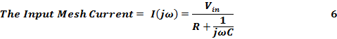
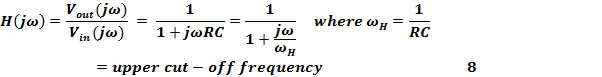
Figure 5. Frequency Domain Response of LPF.

In Figure 4 for cases T ~ τ, we get RISE TIME and FALL TIME at the LEADING and LAGGING EDGE of the Square Wave.

Rise Time = t _r = time taken to rise from 10% of the peak value of the square wave to 90% of the peak value of the square wave at the leading edge.

Similarly Fall Time = t _{f =} time taken to fall from 90% of the peak value of the square wave to 10% of the peak value of the square wave at lagging edge.

It can be shown that:

Thus from Time Domain Studies the frequency Band-Width of a System can be calculated directly without going through the rigour of drawing the Frequency Response Graphs.

APPENDIX: Frequency Spectrum of Infinite Pulse Train.

Figure A. Frequency Spectrum of an Infinite Pulse Train.

In Figure A, in upper half an infinite pulse train is depicted with Pulse Repetition Frequency(PRF) of (1/T) Hz where T= time period of periodicity and τ is the pulse duration and τ/T is duty cycle. In Square wave duty cycle is 50%. In the pulse train shown above T=4τ. As can be seen in the Fourier Series Expansion of the infinite pulse train, the DC spectral component is the mean value (V _p τ/T) and the fundamental frequency component (1/T Hz) and the harmonics spectral component magnitude follows the envelope described by Sinc(θ)= [Sin(θ)/θ ] where θ= [2πn(τ/T)]where n=1,2,3....integers. The Sinc Envelope experiences the first Zero-cross over at frequency = 1/τ and second cross-over at 2/τ.

This means Fourier Spectral Components has a main lobe of frequency components and side-lobes of frequency components. As long as the System’s BW accommodates the main lobe we will get near-faithful reproduction of the pulse train. But if the main lobe gets suppressed then the pulse train will be completely lost.

In LPF, when T<<τ then the fundamental 1/T is>>first cross-over frequency hence the main lobe is completely suppressed and the square wave is completely lost. What is left after filtering is the DC component since it is direct-coupled system.

Similarly in HPF, when T>>τ then the fundamental 1/T<<1/τ and since it is HPF hence the main lobe gets completely suppressed. What is left are the spikes corresponding to the edges of the pulse train. The pulse train itself is completely lost..