0.9 Appendix c

Structure and spectral description

The focus of this technical note is on the decomposition of an FDM signal into its constituent narrowband components. As we have seen, the use of the right assumptions allows digital implementation of this operation to be done very efficiently with an FDM-to-TDM transmultiplexer. In practice, there are applications in which it is desirable to perform the converse operation - combine multiple narrowband signals into an FDM composite. As might be expected, if suitable simplifying assumptions are made, some of the same efficiencies that lead to the FDM-to-TDM transmultiplexer allow the formulation of a TDM-to-FDM transmultiplexer. This appendix demonstrates how this is done. For simplicity, the architecture shown here uses complex-valued input signals and produces a complex-valued output signal.

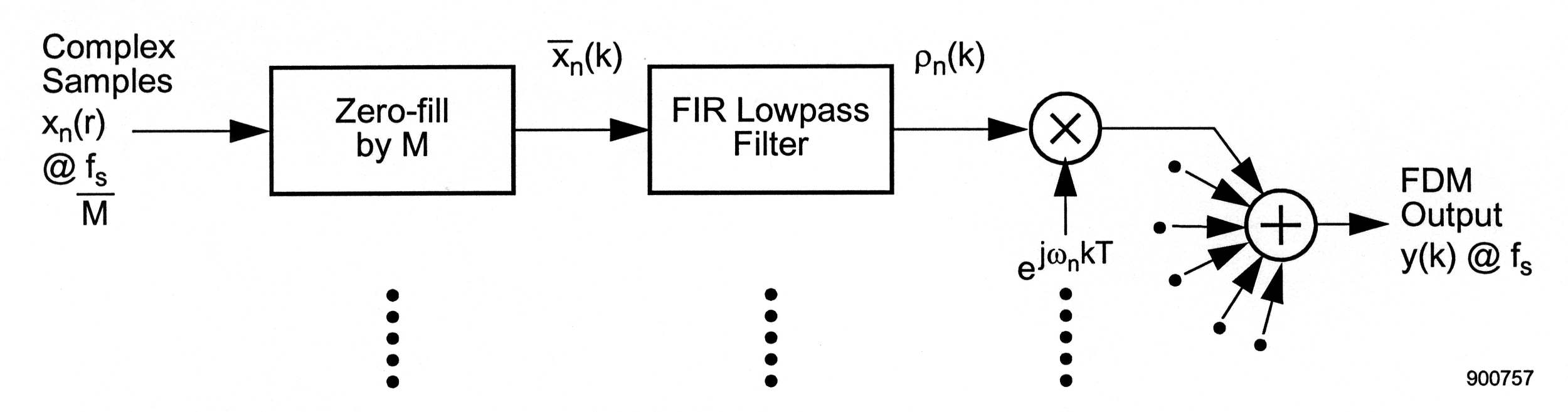
The block diagram of a digitally implemented frequency-division multiplexer is shown in [link] . Each input signal, denoted $x_n\left(r\right)$ , is complex-valued and sampled at a rate of $\frac{f_s}{M}$ . It is zero-filled by the factor M to produce the sequence ${\overline{x}}_n\left(k\right)$ and then lowpass-filtered to produce the interpolated sequence ${\rho }_n\left(k\right)$ . This interpolated sequence is then upconverted by ω _n and then added with other similarly processed inputs to produce the FDM output $y\left(k\right)$ .

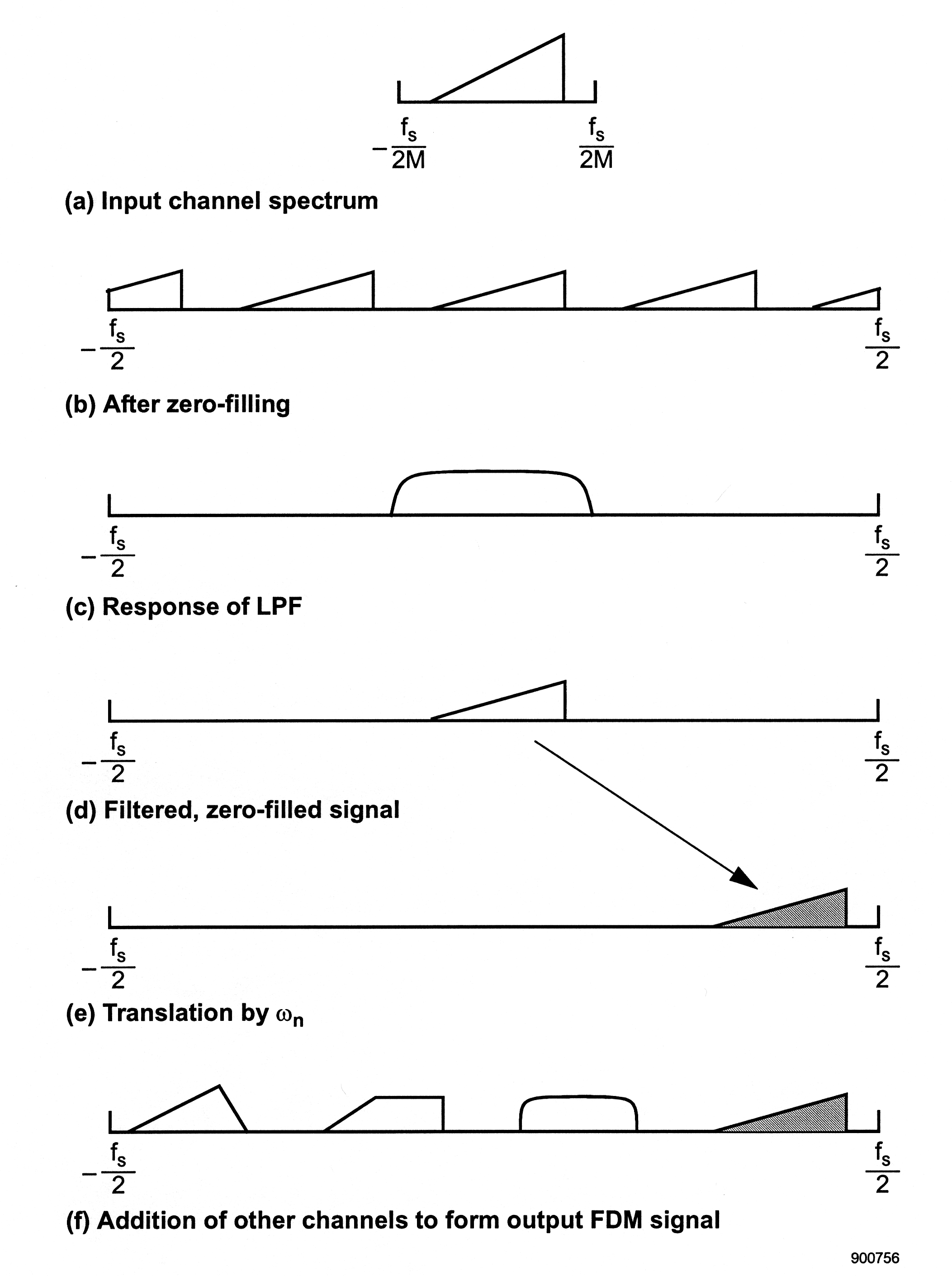
The spectral implications of these steps are shown in [link] . We start by assuming that the narrowband input signal's spectrum is as shown in [link] (a). The zero-filling process creates $M-1$ additional images of the input spectrum and expands the sampling rate to f _s Hz. A properly designed lowpass filter removes the images created by the zero-filling, leaving only the original image centered at DC, shown in [link] (d). Multiplication by $e^{j{\omega }_{n}kT}$ translates the signal so that it is centered at ω _n Hz. If the other translation frequencies are chosen so that the other upconverted input signals do not overlap, then the situation shown in [link] (f) results, that is, the separate input narrowband signals all appear in the single composite output $y\left(k\right)$ , but in disjoint spectral bands.

Mathematical description of equations

We now develop a set that describes the block diagram shown in [link] . The zero-filled input ${\overline{x}}_n\left(k\right)$ is given by

that is, ${\overline{x}}_n\left(k\right)$ equals $x_n\left(r\right)$ when $k=Mr$ but equals 0 otherwise. If we write k as $k\equiv rM+p$ , with p ranging from 0 to $M-1$ , then we see that ${\overline{x}}_n\left(k\right)$ equals zero unless $p=0$ .

The next step is the lowpass filtering of the zero-filled sequence. Denote the pulse response of this filter, as usual, by $h\left(\ell \right)$ , where ℓ runs from 0 to $L-1$ , and L is the pulse response duration. With no loss of generality we can assume that L is an integer multiple of M , the interpolation factor, and therefore that there exists some positive integer Q that satisfies the equation $L\equiv \overline{Q}M$ . This in turn allows ℓ , the running index of the pulse response, to be written as $\ell =qM+v$ , where the integer q runs from 0 to $\overline{Q}-1$ and the integer $v$ runs from 0 to $M-1$ .

The output of the lowpass interpolation filter ${\rho }_n\left(k\right)$ is given by the expression