

| << Chapter < Page | Chapter >> Page > |
Flat fading occurs when
there are obstacles moving in the path between the transmitterand receiver or when the transmitter and receiver are
moving with respect to each other. It ismost commonly modelled as a time-varying channel gain
that attenuates the received signal.The modifier “flat” implies that the loss in gain is
uniform over all frequencies.
In communications jargon,
it is not
frequency selective . This section begins by studying the loss of performance
caused by a time-varying channel gain (using a modifiedversion of
idsys.m ) and then examines the ability of
an adaptive element (the automatic gain control, AGC)to make things right.
In the ideal system of the preceding section, the gain
between the transmitter and the receiver wasimplicitly assumed to be unity.
What happens when this assumptionis violated, when flat fading is experienced in midmessage?
To examine this question, suppose that the channel gainis unity for the first 20% of the transmission,
but that for the last 80% it drops by half.This flat fade can easily be studied by inserting
the following code between the transmitterand the receiver parts of
idsys.m .
lr=length(r);                % length of transmitted signal vector
fp=[ones(1,floor(0.2*lr)),...    0.5*ones(1,lr-floor(0.2*lr))];  % flat fading profiler=r.*fp;                     % apply profile to transmitted signal vector

idsysmod1.m  modification of
idsys.m  with time-varying fading channel
(download file)
The resulting plot of the soft decisions in
[link] (via
plot([1:length(z)], z,'.') )
shows the effect of the fade in the latter 80% of the response.
Shrinking the magnitude of the symbols
by half puts it in the
decision region for
, which generates a large number
of symbol errors. Indeed, the recovered message looks nothinglike the original.
[link] has already introduced
an adaptive element designed to compensate for flat fading:the automatic gain control, which acts to
maintain the power of a signal at a constant knownlevel.
Stripping out the AGC code from
agcvsfading.m >and combining it with
the fading channel just discussed creates a simulation inwhich the fade occurs, but in which the AGC can actively
work to restore the power of the received signalto its desired nominal value
ds
.
ds=pow(r);                      % desired average power of signal
lr=length(r);                   % length of transmitted signal vectorfp=[ones(1,floor(0.2*lr)),...
    0.5*ones(1,lr-floor(0.2*lr))];  % flat fading profile
r=r.*fp;                        % apply profile to transmitted signal vectorg=zeros(1,lr); g(1)=1;          % initialize gain
nr=zeros(1,lr);mu=0.0003;
% stepsizefor i=1:lr-1
% adaptive AGC element  nr(i)=g(i)*r(i);
% AGC output  g(i+1)=g(i)-mu*(nr(i)^2-ds);
% adapt gainend
r=nr;                           % received signal is still called r

idsysmod2.m  modification of
idsys.m
(download file) with fading plus automatic gain control
Inserting this segment into
idsys.m (immediately after the time-varying fading
channel modification) results in only a small number of errorsthat occur right at the time of the fade. Very quickly,
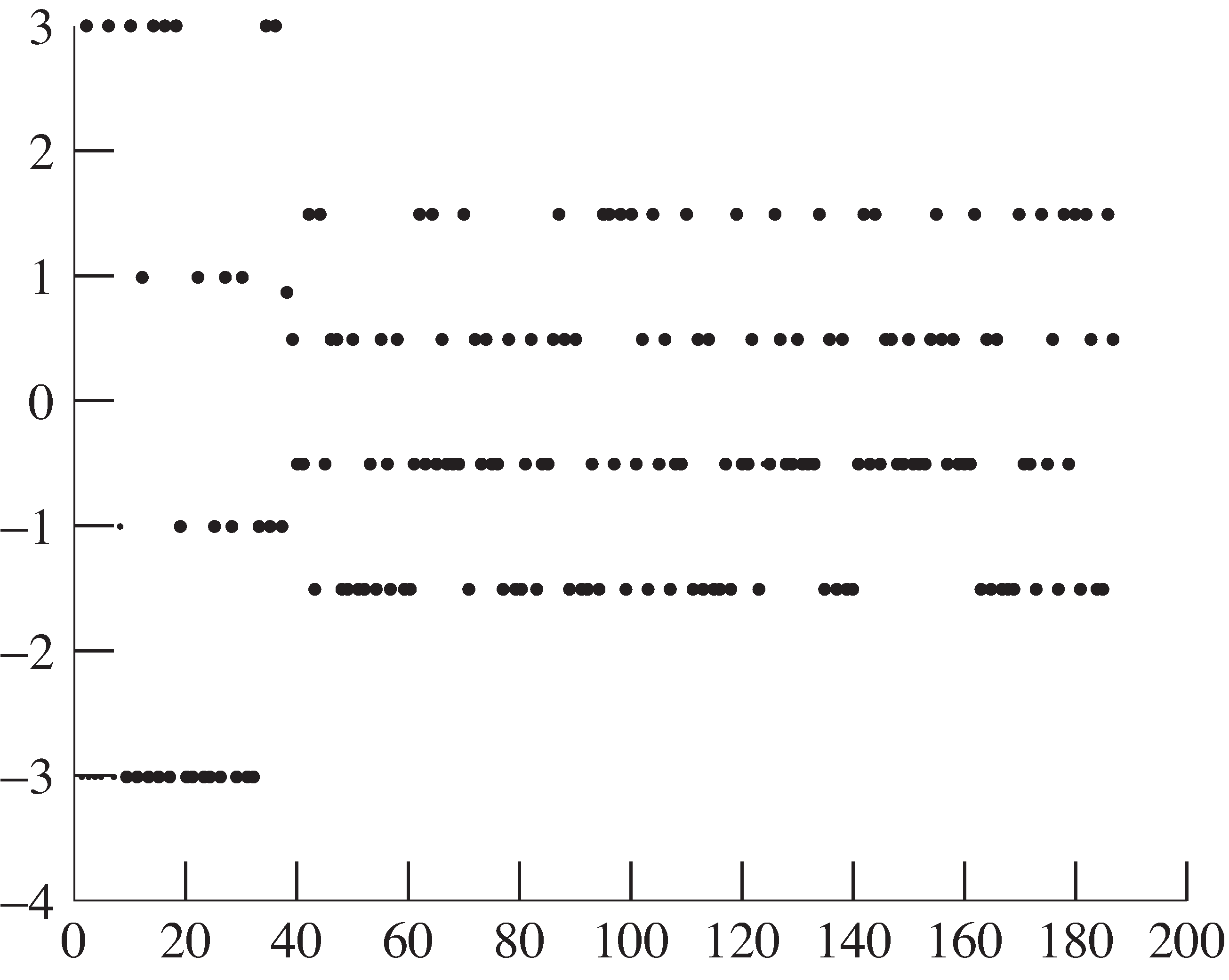
the AGC kicks in to restore the received power.The resulting plot of the soft decisions
(via
plot([1:length(z)],z,'.') ) in
[link] shows how quickly after the abrupt fade the soft decisions
return to the appropriate sector. (Look for where thelarger soft decisions exceed a magnitude of 2.)
Notification Switch
Would you like to follow the 'Software receiver design' conversation and receive update notifications?

|
|

|
|

|
|

|
|

|
|

|
|

|
|

|
|
|
|
|

|