0.6 Regularity, moments, and wavelet system design  (Page 8/13)

Vanishing scaling function moments

While the moments of the wavelets give information about flatness of $H\left(\omega \right)$ and smoothness of $\psi \left(t\right)$ , the moments of $\phi \left(t\right)$ and $h\left(n\right)$ are measures of the “localization" and symmetry characteristics of the scaling function and, therefore, the wavelet transform. We know from [link] that ${\sum }_{n}h\left(n\right)=\sqrt{2}$ and, after normalization, that $\int \phi \left(t\right)dt=1$ . Using [link] , one can show [link] that for $K\ge 2$ , we have

This can be seen in [link] . A generalization of this result has been developed by Johnson [link] and is given in [link] through [link] .

A more general picture of the effects of zero moments can be seen by next considering two approximations. Indeed, this analysis gives a veryimportant insight into the effects of zero moments. The mixture of zero scaling function moments with other specifications is addressed laterin [link] .

Approximation of signals by scaling function projection

The orthogonal projection of a signal $f\left(t\right)$ on the scaling function subspace $V_j$ is given and denoted by

which gives the component of $f\left(t\right)$ which is in $V_j$ and which is the best least squares approximation to $f\left(t\right)$ in $V_j$ .

As given in [link] , the ${\ell }^{th}$ moment of $\psi \left(t\right)$ is defined as

We can now state an important relation of the projection [link] as an approximation to $f\left(t\right)$ in terms of the number of zero wavelet moments and the scale.

Theorem 25 If $m_1\left(\ell \right)=0$ for $\ell =0,1,\cdots ,L$ then the $L^2$ error is

where $C$ is a constant independent of $j$ and $L$ but dependent on $f\left(t\right)$ and the wavelet system [link] , [link] .

This states that at any given scale, the projection of the signal on the subspace at that scale approaches the function itself as the numberof zero wavelet moments (and the length of the scaling filter) goes to infinity. It also states that for any given length, the projection goesto the function as the scale goes to infinity. These approximations converge exponentially fast. This projection is illustrated in [link] .

Approximation of scaling coefficients by samples of the signal

A second approximation involves using the samples of $f\left(t\right)$ as the inner product coefficients in the wavelet expansion of $f\left(t\right)$ in [link] . We denote this sampling approximation by

and the scaling function moment by

and can state [link] the following

Theorem 26 If $m\left(\ell \right)=0$ for $\ell =1,2,\cdots ,L$ then the $L^2$ error is

where $C_2$ is a constant independent of $j$ and $L$ but dependent on $f\left(t\right)$ and the wavelet system.

This is a similar approximation or convergence result to the previous theorem but relates the projection of $f\left(t\right)$ on a $j$ -scale subspace to the sampling approximation in that same subspace. These approximationsare illustrated in [link] .

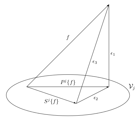
This “vector space" illustration shows the nature and relationships of the two types of approximations. The use of samples as inner productsis an approximation within the expansion subspace $V_j$ . The use of a finite expansion to represent a signal $f\left(t\right)$ is an approximation from $L^2$ onto the subspace $V_j$ . Theorems  [link] and [link] show the nature of those approximations, which, for wavelets, is very good.