

| << Chapter < Page | Chapter >> Page > |
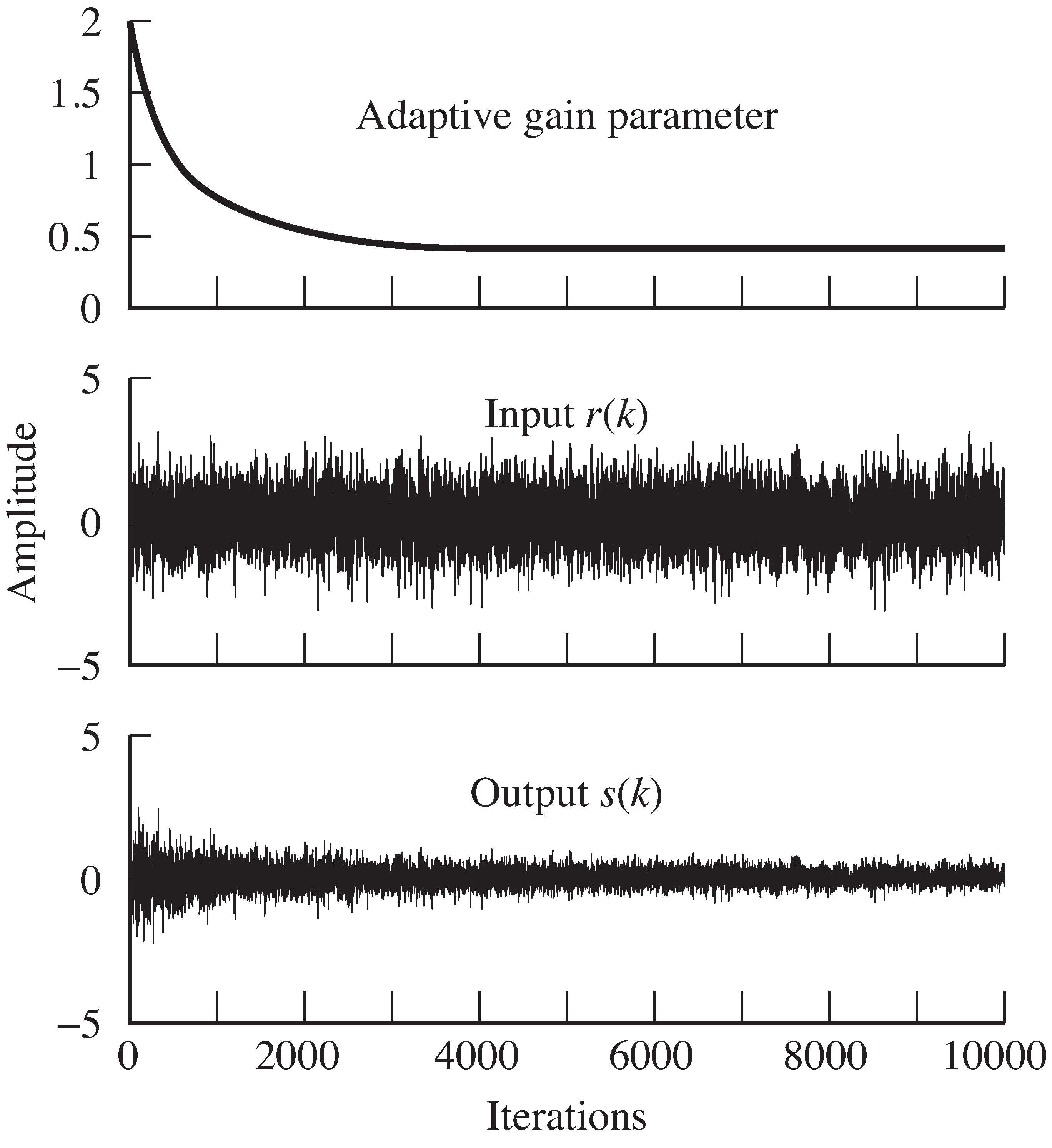
Typical output of
agcgrad.m is shown in
[link] .
The gain parameter
a adjusts automatically to make the
overall power of the output
s roughly equal to the specified
parameter
ds . Using the default values above,
where the average power of
is approximately 1, we find that
converges to about
since
.
The objective
can be implemented similarly by replacing the
avec calculation inside the
for loop with
avec=[(s(k)^2-ds)*(s(k)^2)/a(k),avec(1:end-1)];
In this case, with the default values, converges to about , which is the value that minimizes the least square objective . Thus, the answer which minimizes is different from the answer which minimizes ! More on this later.
As it is easy to see when playing with the
parameters in
agcgrad.m , the size of the averaging parameter
lenavg is relatively unimportant. Even with
lenavg=1 , the algorithms converge and perform approximately
the same! This is because the algorithm updatesare themselves in the form of a lowpass filter.
Removing the averaging from the update gives the simpler formfor
a(k+1)=a(k)-mu*sign(a(k))*(s(k)^2-ds);
or, for ,
a(k+1)=a(k)-mu*(s(k)^2-ds)*(s(k)^2)/a(k);
Try them!
Perhaps the best way to formally describe how the algorithms work is to plot the performance functions.But it is not possible to directly plot or , since they depend on the data sequence . What is possible (and often leads to useful insights)is to plot the performance function averaged over a number of data points (also called the error surface ). As long as the stepsize is small enough and the average is long enough,the mean behavior of the algorithm will be dictated by the shape of the errorsurface in the same way that the objective function of the exact steepest descent algorithm (for instance, the objectives [link] and [link] ) dictate the evolution of the algorithms [link] and [link] .
The following code
agcerrorsurf.m shows how
to calculate the error surface for
:
The variable
n specifies the number of terms
to average over, and
tot sums up the behavior of
the algorithm for all
updates at each possible
parameter value
a . The average of these (
tot/n )
is a close (numerical) approximation to
of
[link] .
Plotting over all
gives the error surface.
n=10000;                       % number of steps in simulation
r=randn(n,1);                  % generate random inputsds=0.15;                       % desired power of output
range=[-0.7:0.02:0.7];         % range specifies range of values of a
Jagc=zeros(size(range));j=0;
for a=range                    % for each value a  j=j+1;
  tot=0;  for i=1:n
    tot=tot+abs(a)*((1/3)*a^2*r(i)^2-ds);  % total cost over all possibilities  end
  Jagc(j)=tot/n;               % take average value, and saveend

agcerrorsurf.m  draw the error surface for the AGC
(download file)
Similarly, the error surface for can be plotted using
tot=tot+0.25*(a^2*r(i)^2-ds)^2; % error surface for JLS
The output of
agcerrorsurf.m for both objective functions
is shown in
[link] .
Observe that zero (which is acritical point of the error surface) is a local maximum
in both cases.The final converged answers (
for
and
for
)
occur at minima. Were the algorithm to be initializedimproperly to a negative value, then it would converge to
the negative of these values.As with the algorithms in
[link] ,
examination of the error surfaces shows
why the algorithms converge as they do.
The parameter
descends the error surface until it can go no
further.
Notification Switch
Would you like to follow the 'Software receiver design' conversation and receive update notifications?

|
|

|
|

|
|

|
|

|
|

|
|
|
|
|

|
|

|
|

|