We return to the topic of classification, and we assume an input
(feature) space
and a binary output (label) space
. Recall that the Bayes classifier (which minimizes the
probability of misclassification) is defined by
Throughout this section, we will denote the conditional probability
function by
Plug-in classifiers
One way to construct a classifier using the training data
is to estimate
and then plug-it
into the form of the Bayes classifier. That is obtain an estimate,
and then form the “plug-in" classification rule
The function
is generally more complicated than
the ultimate classification rule (binary-valued), as we cansee
Therefore, in this sense plug-in methods are solving a more complicated
problem than necessary. However, plug-in methods can perform well,as demonstrated by the next result.
Theorem
Plug-in classifier
Let
be an approximation to
, and consider the plug-in
rule
Then,
where
Consider any
. In proving the optimality of the
Bayes classifier
in
Lecture 2 , we showed that
which is
equivalent to
since
whenever
.
Thus,
where the first inequality follows from the fact
and the second inequality is simply a result of the fact that
is either 0 or 1.
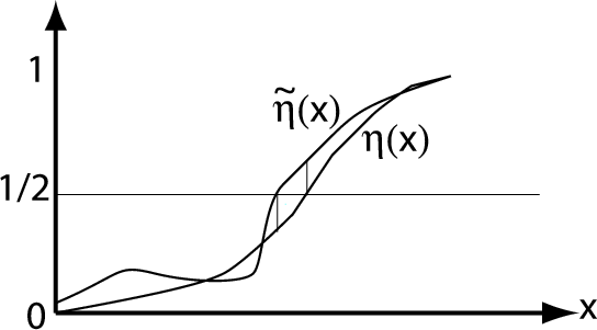
Pictorial illustration of
when
. Note that the
inequality
shows
that the excess risk is at most twice the integral over the setwhere
. The difference
may be arbitrarily large away from
this set without effecting the error rate of the classifier. Thisillustrates the fact that estimating
well everywhere (i.e.,
regression) is unnecessary for the design of a good classifier (weonly need to determine where
crosses the
-level). In
other words, “classification is easier than regression.”
The theorem shows us that a good estimate of
can produce a good
plug-in classification rule. By “good" estimate, we mean an estimator
that is close to
in expected
.
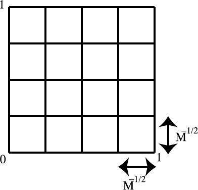
The histogram classifier
Let's assume that the (input) features are randomly distributed over
theunit hypercube
(note that by scaling and
shifting any set of bounded features we can satisfy this assumption),and assume that the (output) labels are binary, i.e.,
. A histogram classifier is based on a partition the hypercube
into
smaller cubes of equal size.
Partition of hypercube in 2 dimensions
Consider the unit square
and partition it into
subsquares of equal area (assuming
is a squared integer). Let
the subsquares be denoted by
.
Example of hypercube
in
equally sized
partition
Define the following
piecewise-constant estimator of
:
where
Like our previous denoising examples, we expect that the bias of
will decrease as
increases, but the variance will
increase as
increases.