

| << Chapter < Page | Chapter >> Page > |
Consider the following setting. Let
where X is a random variable (r.v.) on , is a r.v. on independent of and satisfying
Finally let be a function satisfying
where is a constant. A function satisfying condition [link] is said to be Lipschitz on . Notice that such a function must be continuous, but it is not necessarilydifferentiable. An example of such a function is depicted in [link] (a).

Note that
Consider our usual setup: Estimate using training examples
where means independently and identically distributed . [link] (a) illustrates this setup.
In many applications we can sample as we like, and not necessarily at random. For example we can take samples uniformly on [0,1]
We will proceed with this setup (as in [link] (b)) in the rest of the lecture.
Our goal is to find such that (here is the usual -norm; i.e., ).
Let
The Riskis defined as
The Expected Risk (recall that ourestimator is based on and hence is a r.v.) is defined as
Finally the Empirical Riskis defined as
Let be a sequence of integers satisfying as , and for some integer . That is, for each value of there is an associated integer value . Define the Sieve
is the space of functions that are constant on intervals
From here on we will use and instead of and (dropping the subscript ) for notational ease. Define
Note that .
Upper bound .
The above implies that since . In words, with sufficiently large we can approximate to arbitrary accuracy using models in (even if the functions we are using to approximate are not Lipschitz!).
For any we have
Let Then
Show [link] .
Note that and therefore . Lets analyze now the expected risk of :
where the final step follows from the fact that . A couple of important remarks pertaining the right-hand-side of equation [link] : The first term, , corresponds to the approximation error, and indicates how well can we approximate the function with a function from . Clearly, the larger the class is, the smallest we can make this term. This term is precisely the squared bias of the estimator . The second term, , is the estimation error, the variance of our estimator. We will see that the estimation erroris small if the class of possible estimators is also small.
The behavior of the first term in [link] was already studied. Consider the other term:
Combining all the facts derived we have
This equation used Big-O notation.
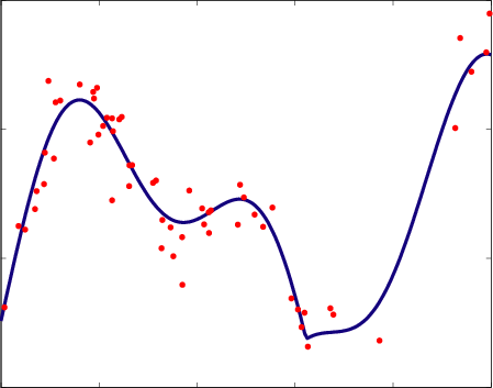
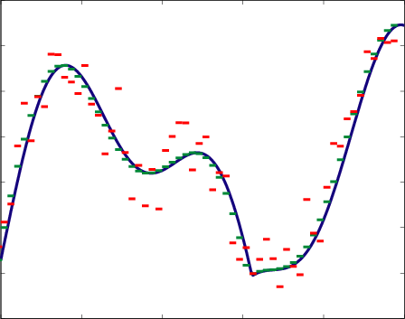
What is the best choice of ? If is small then the approximation error ( i.e., ) is going to be large, but the estimation error ( i.e., ) is going to be small, and vice-versa. This two conflicting goals provide a tradeoff that directs our choice of (as a function of ). In [link] we depict this tradeoff. In [link] (a) we considered a large value, and we see that the approximation of by a function in the class can be very accurate (that is, our estimate will have a small bias), but when we use the measured dataour estimate looks very bad (high variance). On the other hand, as illustrated in [link] (b), using a very small allows our estimator to get very close to the best approximating function in the class , so we have a low variance estimator, but the bias of our estimator ( i.e., the difference between and ) is quite considerable.

We need to balance the two terms in the right-hand-side of [link] in order to maximize the rate of decay (with ) of the expected risk. This implies that therefore and the Mean Squared Error (MSE) is
So the sieve with
produces a -consistent estimator for .
It is interesting to note that the rate of decay of the MSE we obtainwith this strategy cannot be further improved by using more sophisticated estimation techniques (that is, is the minimax MSE rate for this problem). Also, rather surprisingly, we are considering classes of models that are actually not Lipschitz, therefore our estimator of is not a Lipschitz function, unlike itself.
Notification Switch
Would you like to follow the 'Statistical learning theory' conversation and receive update notifications?

|
|

|
|

|
|

|
|

|
|

|
|

|
|

|
|

|
|

|