<< Chapter < Page Chapter >> Page >
Background on a few adaptive filtering algorithms we tried in our echo cancellation project.

Adaptive filtering

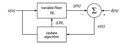
Adaptive filters are time-varying filters that use an update algorithm to create a finite impulse response (FIR) filter that outputs the best approximation of desired signal. Adaptive filters take in a desired signal and an input signal and update their parameters using feedback driven by the error signal. The adaptive filter finds the ideal filter coefficients for a filter that gives the least mean square of the error signal. The error signal is defined as the difference of the desired signal and the output signal.

e ( n ) = d ( n ) y ( n ) MathType@MTEF@5@5@+= feaagGart1ev2aqatCvAUfeBSjuyZL2yd9gzLbvyNv2CaerbuLwBLnhiov2DGi1BTfMBaeXatLxBI9gBaerbd9wDYLwzYbItLDharqqtubsr 4rNCHbGeaGqiVu0Je9sqqrpepC0xbbL8F4rqqrFfpeea0xe9Lq=Jc9vqaqpepm0xbba9pwe9Q8fs0=yqaqpepae9pg0FirpepeKkFr0xfr=x fr=xb9adbaqaaeGaciGaaiaabeqaamaabaabaaGcbaGaamyzaiaacIcacaWGUbGaaiykaiabg2da9iaadsgacaGGOaGaamOBaiaacMcacqGH sislcaWG5bGaaiikaiaad6gacaGGPaaaaa@419E@

At every iteration (or block of samples) the gradient of the mean square error at that time is found, and is then used to adjust the filter coefficients at the time to converge towards the ideal filter coefficients.

adaptive filter block diagram
Adaptive filtering block diagram

We trained adaptive filters using signals recorded in a low-echo environment using three algorithms to filter out echoes in an echoic room and in the OEDK classroom. Our desired signal is a recording of our signal in a low-echo environment that would give us a signal with minimal echo. This gave us a baseline for the distortion of the signal caused by our equipment.

Having gathered a baseline signal, we recorded our input signals in the echoic room and the OEDK classroom. The basic idea of the adaptive filter method is to take in a desired signal and an input signal and mimic an ideal filter with ideal filter coefficients that would make the output signal virtually echo-free and therefore comparable to the desired signal. We explored three different adaptive filtering algorithms for our project.

The least mean squares (lms) algorithm

The LMS algorithm is a class of adaptive filter used to mimic a desired filter by finding the filter coefficients that relate to producing the least mean squares of the error signal (the difference between the desired and the actual signal). The algorithm begins by assuming small weights (zero in most cases), and at each step, by finding the gradient of the mean square error, E [ e 2 ( n ) ] MathType@MTEF@5@5@+= feaagGart1ev2aqatCvAUfeBSjuyZL2yd9gzLbvyNv2CaerbuLwBLnhiov2DGi1BTfMBaeXatLxBI9gBaerbd9wDYLwzYbItLDharqqtubsr 4rNCHbGeaGqiVu0Je9sqqrpepC0xbbL8F4rqqrFfpeea0xe9Lq=Jc9vqaqpepm0xbba9pwe9Q8fs0=yqaqpepae9pg0FirpepeKkFr0xfr=x fr=xb9adbaqaaeGaciGaaiaabeqaamaabaabaaGcbaaeaaaaaaaaa8qacaWGfbGaai4waiaadwgapaWaaWbaaSqabeaapeGaaGOmaaaakiaa cIcacaWGUbGaaiykaiaac2faaaa@3CE8@ , the weights are updated using this cost function. Each iteration uses three steps:

  • Calculate the output of the filter.
y ( n ) = w T ( n ) x ( n ) MathType@MTEF@5@5@+= feaagGart1ev2aqatCvAUfeBSjuyZL2yd9gzLbvyNv2CaerbuLwBLnhiov2DGi1BTfMBaeXatLxBI9gBaerbd9wDYLwzYbItLDharqqtubsr 4rNCHbGeaGqiVu0Je9sqqrpepC0xbbL8F4rqqrFfpeea0xe9Lq=Jc9vqaqpepm0xbba9pwe9Q8fs0=yqaqpepae9pg0FirpepeKkFr0xfr=x fr=xb9adbaqaaeGaciGaaiaabeqaamaabaabaaGcbaaeaaaaaaaaa8qacaWG5bGaaiikaiaad6gacaGGPaGaeyypa0Jaam4DamaaCaaaleqa baGaamivaaaakiaacIcacaWGUbGaaiykaiaadIhacaGGOaGaamOBaiaacMcaaaa@4207@
  • Calculate the estimate of the error using the error signal.
e ( n ) = d ( n ) y ( n ) MathType@MTEF@5@5@+= feaagGart1ev2aqatCvAUfeBSjuyZL2yd9gzLbvyNv2CaerbuLwBLnhiov2DGi1BTfMBaeXatLxBI9gBaerbd9wDYLwzYbItLDharqqtubsr 4rNCHbGeaGqiVu0Je9sqqrpepC0xbbL8F4rqqrFfpeea0xe9Lq=Jc9vqaqpepm0xbba9pwe9Q8fs0=yqaqpepae9pg0FirpepeKkFr0xfr=x fr=xb9adbaqaaeGaciGaaiaabeqaamaabaabaaGcbaGaamyzaiaacIcacaWGUbGaaiykaiabg2da9iaadsgacaGGOaGaamOBaiaacMcacqGH sislcaWG5bGaaiikaiaad6gacaGGPaaaaa@419E@
  • Update the weights of the FIR coefficients.
w ( n + 1 ) = w ( n ) + 2 μ e ( n ) x ( n ) MathType@MTEF@5@5@+= feaagGart1ev2aqatCvAUfeBSjuyZL2yd9gzLbvyNv2CaerbuLwBLnhiov2DGi1BTfMBaeXatLxBI9gBaerbd9wDYLwzYbItLDharqqtubsr 4rNCHbGeaGqiVu0Je9sqqrpepC0xbbL8F4rqqrFfpeea0xe9Lq=Jc9vqaqpepm0xbba9pwe9Q8fs0=yqaqpepae9pg0FirpepeKkFr0xfr=x fr=xb9adbaqaaeGaciGaaiaabeqaamaabaabaaGcbaaeaaaaaaaaa8qacaWG3bGaaiikaiaad6gacqGHRaWkcaaIXaGaaiykaiabg2da9iaa dEhacaGGOaGaamOBaiaacMcacqGHRaWkcaaIYaGaeqiVd0MaamyzaiaacIcacaWGUbGaaiykaiaadIhacaGGOaGaamOBaiaacMcaaaa@491C@
y ( n ) MathType@MTEF@5@5@+= feaagGart1ev2aqatCvAUfeBSjuyZL2yd9gzLbvyNv2CaerbuLwBLnhiov2DGi1BTfMBaeXatLxBI9gBaerbd9wDYLwzYbItLDharqqtubsr 4rNCHbGeaGqiVu0Je9sqqrpepC0xbbL8F4rqqrFfpeea0xe9Lq=Jc9vqaqpepm0xbba9pwe9Q8fs0=yqaqpepae9pg0FirpepeKkFr0xfr=x fr=xb9adbaqaaeGaciGaaiaabeqaamaabaabaaGcbaaeaaaaaaaaa8qacaWG5bGaaiikaiaad6gacaGGPaaaaa@3960@ is the output of the filter, w ( n ) MathType@MTEF@5@5@+= feaagGart1ev2aqatCvAUfeBSjuyZL2yd9gzLbvyNv2CaerbuLwBLnhiov2DGi1BTfMBaeXatLxBI9gBaerbd9wDYLwzYbItLDharqqtubsr 4rNCHbGeaGqiVu0Je9sqqrpepC0xbbL8F4rqqrFfpeea0xe9Lq=Jc9vqaqpepm0xbba9pwe9Q8fs0=yqaqpepae9pg0FirpepeKkFr0xfr=x fr=xb9adbaqaaeGaciGaaiaabeqaamaabaabaaGcbaaeaaaaaaaaa8qacaWG3bGaaiikaiaad6gacaGGPaaaaa@395E@ are the coefficients of the FIR filter, x ( n ) MathType@MTEF@5@5@+= feaagGart1ev2aqatCvAUfeBSjuyZL2yd9gzLbvyNv2CaerbuLwBLnhiov2DGi1BTfMBaeXatLxBI9gBaerbd9wDYLwzYbItLDharqqtubsr 4rNCHbGeaGqiVu0Je9sqqrpepC0xbbL8F4rqqrFfpeea0xe9Lq=Jc9vqaqpepm0xbba9pwe9Q8fs0=yqaqpepae9pg0FirpepeKkFr0xfr=x fr=xb9adbaqaaeGaciGaaiaabeqaamaabaabaaGcbaaeaaaaaaaaa8qacaWG4bGaaiikaiaad6gacaGGPaaaaa@395F@ is the input signal, d ( n ) MathType@MTEF@5@5@+= feaagGart1ev2aqatCvAUfeBSjuyZL2yd9gzLbvyNv2CaerbuLwBLnhiov2DGi1BTfMBaeXatLxBI9gBaerbd9wDYLwzYbItLDharqqtubsr 4rNCHbGeaGqiVu0Je9sqqrpepC0xbbL8F4rqqrFfpeea0xe9Lq=Jc9vqaqpepm0xbba9pwe9Q8fs0=yqaqpepae9pg0FirpepeKkFr0xfr=x fr=xb9adbaqaaeGaciGaaiaabeqaamaabaabaaGcbaGaamizaiaacIcacaWGUbGaaiykaaaa@392B@ is the desired signal, and μ MathType@MTEF@5@5@+= feaagGart1ev2aqatCvAUfeBSjuyZL2yd9gzLbvyNv2CaerbuLwBLnhiov2DGi1BTfMBaeXatLxBI9gBaerbd9wDYLwzYbItLDharqqtubsr 4rNCHbGeaGqiVu0Je9sqqrpepC0xbbL8F4rqqrFfpeea0xe9Lq=Jc9vqaqpepm0xbba9pwe9Q8fs0=yqaqpepae9pg0FirpepeKkFr0xfr=x fr=xb9adbaqaaeGaciGaaiaabeqaamaabaabaaGcbaaeaaaaaaaaa8qacqaH8oqBaaa@37CC@ is the step size.

Computational complexity: 2 N MathType@MTEF@5@5@+= feaagGart1ev2aqatCvAUfeBSjuyZL2yd9gzLbvyNv2CaerbuLwBLnhiov2DGi1BTfMBaeXatLxBI9gBaerbd9wDYLwzYbItLDharqqtubsr 4rNCHbGeaGqiVu0Je9sqqrpepC0xbbL8F4rqqrFfpeea0xe9Lq=Jc9vqaqpepm0xbba9pwe9Q8fs0=yqaqpepae9pg0FirpepeKkFr0xfr=x fr=xb9adbaqaaeGaciGaaiaabeqaamaabaabaaGcbaaeaaaaaaaaa8qacaaIYaGaamOtaaaa@37A5@ additions, 2 N + 1 MathType@MTEF@5@5@+= feaagGart1ev2aqatCvAUfeBSjuyZL2yd9gzLbvyNv2CaerbuLwBLnhiov2DGi1BTfMBaeXatLxBI9gBaerbd9wDYLwzYbItLDharqqtubsr 4rNCHbGeaGqiVu0Je9sqqrpepC0xbbL8F4rqqrFfpeea0xe9Lq=Jc9vqaqpepm0xbba9pwe9Q8fs0=yqaqpepae9pg0FirpepeKkFr0xfr=x fr=xb9adbaqaaeGaciGaaiaabeqaamaabaabaaGcbaaeaaaaaaaaa8qacaaIYaGaamOtaiabgUcaRiaaigdaaaa@3942@ multiplications.

The MathWorks adaptfilt.lms documentation can be used in Matlab to create an LMS adaptive filter object.

The normalized lms (nlms) algorithm

NLMS allows for a variable step size μ ( n ) MathType@MTEF@5@5@+= feaagGart1ev2aqatCvAUfeBSjuyZL2yd9gzLbvyNv2CaerbuLwBLnhiov2DGi1BTfMBaeXatLxBI9gBaerbd9wDYLwzYbItLDharqqtubsr 4rNCHbGeaGqiVu0Je9sqqrpepC0xbbL8F4rqqrFfpeea0xe9Lq=Jc9vqaqpepm0xbba9pwe9Q8fs0=yqaqpepae9pg0FirpepeKkFr0xfr=x fr=xb9adbaqaaeGaciGaaiaabeqaamaabaabaaGcbaaeaaaaaaaaa8qacqaH8oqBcaGGOaGaamOBaiaacMcaaaa@3A18@ for each iteration. The first two steps of the algorithm are identical to the first two steps of the regular LMS algorithm.

  • Calculate the output of the filter.
y ( n ) = w T ( n ) x ( n ) MathType@MTEF@5@5@+= feaagGart1ev2aqatCvAUfeBSjuyZL2yd9gzLbvyNv2CaerbuLwBLnhiov2DGi1BTfMBaeXatLxBI9gBaerbd9wDYLwzYbItLDharqqtubsr 4rNCHbGeaGqiVu0Je9sqqrpepC0xbbL8F4rqqrFfpeea0xe9Lq=Jc9vqaqpepm0xbba9pwe9Q8fs0=yqaqpepae9pg0FirpepeKkFr0xfr=x fr=xb9adbaqaaeGaciGaaiaabeqaamaabaabaaGcbaaeaaaaaaaaa8qacaWG5bGaaiikaiaad6gacaGGPaGaeyypa0Jaam4DamaaCaaaleqa baGaamivaaaakiaacIcacaWGUbGaaiykaiaadIhacaGGOaGaamOBaiaacMcaaaa@4207@
  • Calculate the estimate of the error using the error signal.
e ( n ) = d ( n ) y ( n ) MathType@MTEF@5@5@+= feaagGart1ev2aqatCvAUfeBSjuyZL2yd9gzLbvyNv2CaerbuLwBLnhiov2DGi1BTfMBaeXatLxBI9gBaerbd9wDYLwzYbItLDharqqtubsr 4rNCHbGeaGqiVu0Je9sqqrpepC0xbbL8F4rqqrFfpeea0xe9Lq=Jc9vqaqpepm0xbba9pwe9Q8fs0=yqaqpepae9pg0FirpepeKkFr0xfr=x fr=xb9adbaqaaeGaciGaaiaabeqaamaabaabaaGcbaGaamyzaiaacIcacaWGUbGaaiykaiabg2da9iaadsgacaGGOaGaamOBaiaacMcacqGH sislcaWG5bGaaiikaiaad6gacaGGPaaaaa@419E@
  • Calculate the step size for the input.
μ ( n ) = 1 x T ( n ) x ( n ) MathType@MTEF@5@5@+= feaagGart1ev2aqatCvAUfeBSjuyZL2yd9gzLbvyNv2CaerbuLwBLnhiov2DGi1BTfMBaeXatLxBI9gBaerbd9wDYLwzYbItLDharqqtubsr 4rNCHbGeaGqiVu0Je9sqqrpepC0xbbL8F4rqqrFfpeea0xe9Lq=Jc9vqaqpepm0xbba9pwe9Q8fs0=yqaqpepae9pg0FirpepeKkFr0xfr=x fr=xb9adbaqaaeGaciGaaiaabeqaamaabaabaaGcbaGaeqiVd0Maaiikaiaad6gacaGGPaGaeyypa0ZaaSaaaeaacaaIXaaabaGaamiEamaa CaaaleqabaGaamivaaaakiaacIcacaWGUbGaaiykaiaadIhacaGGOaGaamOBaiaacMcaaaaaaa@436B@
  • Update the weights of the FIR coefficients.
w ( n + 1 ) = w ( n ) + μ ( n ) e ( n ) x ( n ) MathType@MTEF@5@5@+= feaagGart1ev2aqatCvAUfeBSjuyZL2yd9gzLbvyNv2CaerbuLwBLnhiov2DGi1BTfMBaeXatLxBI9gBaerbd9wDYLwzYbItLDharqqtubsr 4rNCHbGeaGqiVu0Je9sqqrpepC0xbbL8F4rqqrFfpeea0xe9Lq=Jc9vqaqpepm0xbba9pwe9Q8fs0=yqaqpepae9pg0FirpepeKkFr0xfr=x fr=xb9adbaqaaeGaciGaaiaabeqaamaabaabaaGcbaGaam4DaiaacIcacaWGUbGaey4kaSIaaGymaiaacMcacqGH9aqpcaWG3bGaaiikaiaa d6gacaGGPaGaey4kaSIaeqiVd0Maaiikaiaad6gacaGGPaGaamyzaiaacIcacaWGUbGaaiykaiaadIhacaGGOaGaamOBaiaacMcaaaa@4A8C@

Computational Complexity: 2 N MathType@MTEF@5@5@+= feaagGart1ev2aqatCvAUfeBSjuyZL2yd9gzLbvyNv2CaerbuLwBLnhiov2DGi1BTfMBaeXatLxBI9gBaerbd9wDYLwzYbItLDharqqtubsr 4rNCHbGeaGqiVu0Je9sqqrpepC0xbbL8F4rqqrFfpeea0xe9Lq=Jc9vqaqpepm0xbba9pwe9Q8fs0=yqaqpepae9pg0FirpepeKkFr0xfr=x fr=xb9adbaqaaeGaciGaaiaabeqaamaabaabaaGcbaGaaGOmaiaad6eaaaa@3785@ additions 3 N + 1 MathType@MTEF@5@5@+= feaagGart1ev2aqatCvAUfeBSjuyZL2yd9gzLbvyNv2CaerbuLwBLnhiov2DGi1BTfMBaeXatLxBI9gBaerbd9wDYLwzYbItLDharqqtubsr 4rNCHbGeaGqiVu0Je9sqqrpepC0xbbL8F4rqqrFfpeea0xe9Lq=Jc9vqaqpepm0xbba9pwe9Q8fs0=yqaqpepae9pg0FirpepeKkFr0xfr=x fr=xb9adbaqaaeGaciGaaiaabeqaamaabaabaaGcbaGaaG4maiaad6eacqGHRaWkcaaIXaaaaa@3923@ multiplications.

The MathWorks adaptfilt.nlms documentation can be used in Matlab to create an NLMS adaptive filter object.

The block lms (blms) algorithm

Rather than computing by discrete samples, the BLMS algorithm calculates in blocks of data, reducing computation cost and improving the convergence rate. The BLMS algorithm can be implemented in the frequency domain using the Discrete Fourier Transform or the FFT.

Computational complexity: 4 N B + ( N B + 3 ) log ( 2 B ) MathType@MTEF@5@5@+= feaagGart1ev2aqatCvAUfeBSjuyZL2yd9gzLbvyNv2CaerbuLwBLnhiov2DGi1BTfMBaeXatLxBI9gBaerbd9wDYLwzYbItLDharqqtubsr 4rNCHbGeaGqiVu0Je9sqqrpepC0xbbL8F4rqqrFfpeea0xe9Lq=Jc9vqaqpepm0xbba9pwe9Q8fs0=yqaqpepae9pg0FirpepeKkFr0xfr=x fr=xb9adbaqaaeGaciGaaiaabeqaamaabaabaaGcbaWaaSaaaeaacaaI0aGaamOtaaqaaiaadkeaaaGaey4kaSYaaeWaaeaadaWcaaqaaiaa d6eaaeaacaWGcbaaaiabgUcaRiaaiodaaiaawIcacaGLPaaaciGGSbGaai4BaiaacEgacaGGOaGaaGOmaiaadkeacaGGPaaaaa@43BE@ , where B MathType@MTEF@5@5@+= feaagGart1ev2aqatCvAUfeBSjuyZL2yd9gzLbvyNv2CaerbuLwBLnhiov2DGi1BTfMBaeXatLxBI9gBaerbd9wDYLwzYbItLDharqqtubsr 4rNCHbGeaGqiVu0Je9sqqrpepC0xbbL8F4rqqrFfpeea0xe9Lq=Jc9vqaqpepm0xbba9pwe9Q8fs0=yqaqpepae9pg0FirpepeKkFr0xfr=x fr=xb9adbaqaaeGaciGaaiaabeqaamaabaabaaGcbaGaamOqaaaa@36BD@ is the block length.

The MathWorks adaptfilt.blms documentation can be used in Matlab to create a BLMS adaptive filter object.

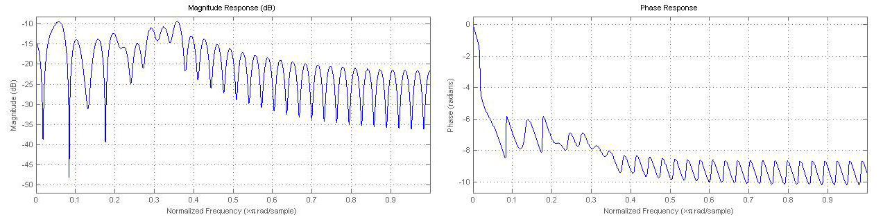
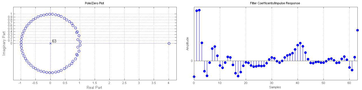
Example of an fir filter created using adaptfilt in matlab

blms filter example blms filter example
This particular filter is a BLMS trained on the male voice signal. Notice that the unit circle is in the region of convergence in the pole/zero plot (the filter is BIBO stable).

Filtering in matlab

  1. Choose a signal to be recorded. We chose a pseudo-dirac, an audiobook recording from The Hunger Games and a recording from Winston Churchill's A History of the English Peoples .
  2. Record the signal being played in a room with desired acoustical properties. This is the desired signal, d ( n ) MathType@MTEF@5@5@+= feaagGart1ev2aqatCvAUfeBSjuyZL2yd9gzLbvyNv2CaerbuLwBLnhiov2DGi1BTfMBaeXatLxBI9gBaerbd9wDYLwzYbItLDharqqtubsr 4rNCHbGeaGqiVu0Je9sqqrpepC0xbbL8F4rqqrFfpeea0xe9Lq=Jc9vqaqpepm0xbba9pwe9Q8fs0=yqaqpepae9pg0FirpepeKkFr0xfr=x fr=xb9adbaqaaeGaciGaaiaabeqaamaabaabaaGcbaGaamizaiaacIcacaWGUbGaaiykaaaa@392B@ . We chose a carpeted room in Hanszen College that had little discernible echo.
  3. Record the signal being played in the echoed room. This is the input signal x ( n ) MathType@MTEF@5@5@+= feaagGart1ev2aqatCvAUfeBSjuyZL2yd9gzLbvyNv2CaerbuLwBLnhiov2DGi1BTfMBaeXatLxBI9gBaerbd9wDYLwzYbItLDharqqtubsr 4rNCHbGeaGqiVu0Je9sqqrpepC0xbbL8F4rqqrFfpeea0xe9Lq=Jc9vqaqpepm0xbba9pwe9Q8fs0=yqaqpepae9pg0FirpepeKkFr0xfr=x fr=xb9adbaqaaeGaciGaaiaabeqaamaabaabaaGcbaGaamiEaiaacIcacaWGUbGaaiykaaaa@393F@ . We recorded in the OEDK classroom and in an even more echoic classroom in Wiess College.
  4. Import both responses into Matlab.
  5. If you use Matlab's built-in adaptive filters. Create the adaptfilt object corresponding to the algorithm with desired parameters.
  6. Use the maxstep() function to check that your filter is stable. If not, adjust your step size.
  7. Use the filter() with your filter object, the input signal and the desire signal.
The desired signal, d ( n ) MathType@MTEF@5@5@+= feaagGart1ev2aqatCvAUfeBSjuyZL2yd9gzLbvyNv2CaerbuLwBLnhiov2DGi1BTfMBaeXatLxBI9gBaerbd9wDYLwzYbItLDharqqtubsr 4rNCHbGeaGqiVu0Je9sqqrpepC0xbbL8F4rqqrFfpeea0xe9Lq=Jc9vqaqpepm0xbba9pwe9Q8fs0=yqaqpepae9pg0FirpepeKkFr0xfr=x fr=xb9adbaqaaeGaciGaaiaabeqaamaabaabaaGcbaGaamizaiaacIcacaWGUbGaaiykaaaa@392B@ , needs to be recorded in another room in order to neutralize the effects of the recording equipment and the amplifier. Using the original signal could lead to the filter trying to compensate for effects introduced by the equipment and the amplifier instead of the echoes caused by the room. Furthermore, the desired and input signals need to start at the same time. Cut out any silence beforehand so that the vectors line up, this way the adaptive filter sifts out the echoes at the appropriate times.
We used the Audacity software to record the sounds, trim the beginning of the sound files, and zero pad them to equal length. We exported these files as .wav files and then, on Matlab, used the wavread() function to import the sounds.
Links to MathWorks documentation for various adaptive filters can be found here .

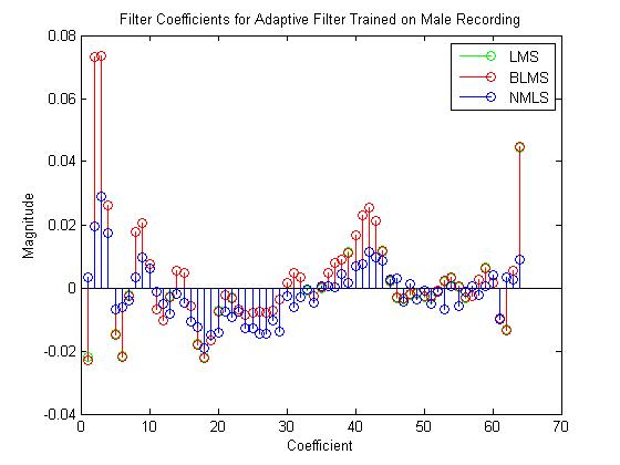
Fir filter coefficients for each algorithm

Stem plot of coefficients
With the same training set (desired signal) each algorithm yields different filter coefficients. Step size: .0006. BLMS block length: 64.

Get Jobilize Job Search Mobile App in your pocket Now!

Get it on Google Play Download on the App Store Now


Source:  OpenStax, Characterization and application of echo cancellation methods. OpenStax CNX. Dec 17, 2012 Download for free at http://cnx.org/content/col11468/1.3
Google Play and the Google Play logo are trademarks of Google Inc.

Notification Switch

Would you like to follow the 'Characterization and application of echo cancellation methods' conversation and receive update notifications?

Ask