

| << Chapter < Page | Chapter >> Page > |
The results from the simulations for the random knock-out runs are displayed in the figures below, which depict the average relative Frobenius-norm error over 25 trials versus fraction of unknown entries.
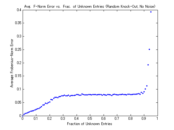
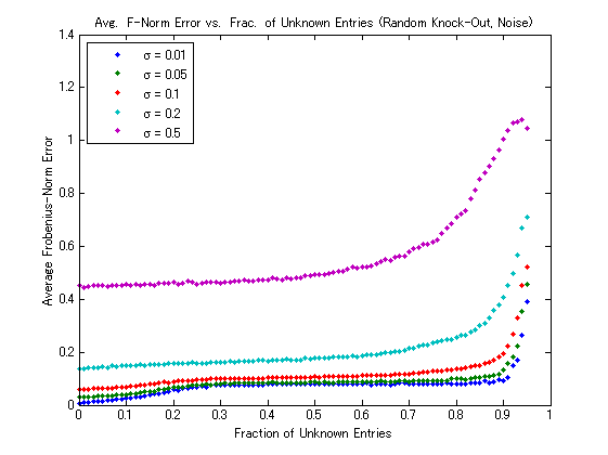
As these two figures illustrate, the results for the random knock-out trials were quite good. As expected, as the fraction of unknown entries becomes large, the error eventually becomes severe, while for very low fractions of unknown entries, the error is extremely small. What is amazing is that for moderate fractions of unknown entries the algorithm still performs remarkably well, and its performance doesn't degrade much by the loss of a few more entries:the graphs are nearly flat over the range from 0.3 to 0.8! As the second figure shows (and as might be imagined), noise only makes the error worse; however, the plot also shows that the algorithm is reasonably robust to noise in that perturbations of the distance data by small amounts of noise don't become magnified into massive errors.
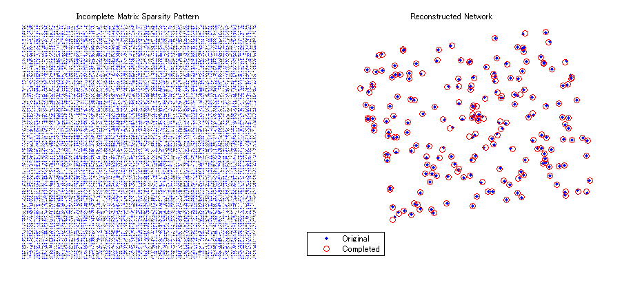
As an example, consider Figure 3 below, which displays the results of a typical no-noise random knock-out run with knock-out probability 0.5. On the left is a plot of the sparsity pattern for the incomplete matrix. A blue dot represents a known entry, while a blank space represents an unknown one. On the right is a plot of what the network looks like after being reconstructed using multidimensional scaling. Observe that the red circles for the networkcorresponding to the network generated by the completed matrix enclose the blue dots of the original network's structure quite well, indicating that the match is very good.
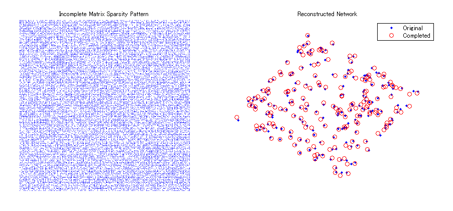
For an illustration of how the results look with noise, see Figure 4 below. This figure shows the results of a typical noise-present random knock-out run with knock-out probability of 0.5 and noise standard deviation 0.05. The agreement in the reconstructed network is not as good as it was for the no-noise case, but the points of the reconstructed network are “clustered" in the right locations, and some of the prominent features of the original networkare present in the reconstructed one as well.
Notification Switch
Would you like to follow the 'A matrix completion approach to sensor network localization' conversation and receive update notifications?

|
|

|
|

|
|

|
|

|
|

|
|

|
|

|
|

|
|

|