<< Chapter < Page Chapter >> Page >
This collection reviews fundamental concepts underlying the use of concise models for signal processing. Topics are presented from a geometric perspective and include low-dimensional linear, sparse, and manifold-based signal models, approximation, compression, dimensionality reduction, and Compressed Sensing.

We now survey some common and important models in signal processing, each of which involves some notion of conciseness tothe signal structure. We see in each case that this conciseness gives rise to a low-dimensional geometry within the ambient signalspace.

Linear models

Some of the simplest models in signal processing correspond to linear subspaces of the ambient signal space. Bandlimited signals are one such example. Supposing, for example,that a 2 π -periodic signal f has Fourier transform F ( ω ) = 0 for | ω | > B , the Shannon/Nyquist sampling theorem  [link] states that such signals can be reconstructed from 2 B samples. Because the space of B -bandlimited signals is closed under addition and scalar multiplication, it follows that the set of such signals forms a 2 B -dimensional linear subspace of L 2 ( [ 0 , 2 π ) ) .

Linear signal models also appear in cases where a model dictates a linear constraint on a signal. Considering a discrete length- N signal x , for example, such a constraint can be written in matrix form as

A x = 0
for some M × N matrix A . Signals obeying such a model are constrained to live in N ( A ) (again, obviously, a linear subspace of R N ).

A very similar class of models concerns signals living in an affine space, which can be represented for a discrete signal using

A x = y .
The class of such x lives in a shifted nullspace x ^ + N ( A ) , where x ^ is any solution to the equation A x ^ = y .

Revisiting the dictionary setting (see Signal Dictionaries and Representations ), one last important linear model arises in cases where we select K specific elements from the dictionary Ψ and then construct signals using linear combinations of only these K elements; in this case the set of possible signals forms a K -dimensional hyperplane in the ambient signal space (see [link] (a)).

Simple models for signals in R 2 . (a) The linear space spanned by one element of the dictionary Ψ . The bold vectors denote the elements of the dictionary, while the dashed line (plus the corresponding dictionary element) denotes the subspace spanned by that dictionary element. (b) The nonlinear set of 1-sparse signals that can be built using Ψ . (c) A manifold M .

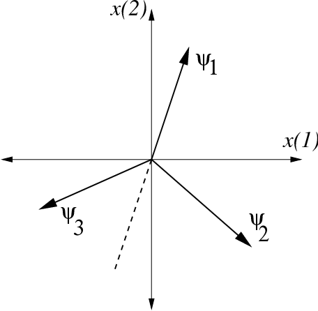
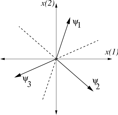
For example, we may construct low-frequency signals using combinations of only the lowest frequency sinusoids from theFourier dictionary. Similar subsets may be chosen from the wavelet dictionary; in particular, one may choose only elements that spana particular scaling space V j . As we have mentioned previously, harmonic dictionaries such as sinusoids and wavelets arewell-suited to representing smooth Lipschitz smoothness We say a continuous-time function of D variables has smoothness of order H > 0 , where H = r + ν , r is an integer, and ν ( 0 , 1 ] , if the following criteria are met [link] , [link] :

  • All iterated partial derivatives with respect to the D directions up to order r exist and are continuous.
  • All such partial derivatives of order r satisfy a Lipschitz condition of order ν (also known as a Hölder condition).(A function d Lip ( ν ) if | d ( t 1 + t 2 ) - d ( t 1 ) | C t 2 ν for all D -dimensional vectors t 1 , t 2 .)
We will sometimes consider the space of smooth functions whose partial derivatives up to order r are bounded by some constant Ω . With somewhat nonstandard notation, we denote the space of such bounded functions with bounded partial derivatives by C H , where this notation carries an implicit dependence on Ω . Observe that r = H - 1 , where · denotes rounding up. Also, when H is an integer C H includes as a subset the space traditionally denoted by the notation “ C H ” (the class of functions that have H = r + 1 continuous partial derivatives).
signals. This can be seen in the decay of their transform coefficients. For example, we canrelate the smoothness of a continuous 1-D function f to the decay of its Fourier coefficients F ( ω ) ; in particular, if | F ( ω ) | ( 1 + | ω | H ) d ω < , then f C H [link] . In order to satisfy | F ( ω ) | ( 1 + | ω | H ) d ω < , a signal must have a sufficiently fast decay of the Fourier transform coefficients | F ( ω ) | as ω grows. Wavelet coefficients exhibit a similar decay for smooth signals:supposing f C H and the wavelet basis function has at least H vanishing moments, then as the scale j , the magnitudes of the wavelet coefficients decayas 2 - j ( H + 1 / 2 ) [link] . (Recall that f C H implies f is well-approximated by a polynomial, and so due the vanishing moments this polynomial will have zero contribution tothe wavelet coefficients.)

Questions & Answers

differentiate between demand and supply giving examples
Lambiv Reply
differentiated between demand and supply using examples
Lambiv
what is labour ?
Lambiv
how will I do?
Venny Reply
how is the graph works?I don't fully understand
Rezat Reply
information
Eliyee
devaluation
Eliyee
t
WARKISA
hi guys good evening to all
Lambiv
multiple choice question
Aster Reply
appreciation
Eliyee
explain perfect market
Lindiwe Reply
In economics, a perfect market refers to a theoretical construct where all participants have perfect information, goods are homogenous, there are no barriers to entry or exit, and prices are determined solely by supply and demand. It's an idealized model used for analysis,
Ezea
What is ceteris paribus?
Shukri Reply
other things being equal
AI-Robot
When MP₁ becomes negative, TP start to decline. Extuples Suppose that the short-run production function of certain cut-flower firm is given by: Q=4KL-0.6K2 - 0.112 • Where is quantity of cut flower produced, I is labour input and K is fixed capital input (K-5). Determine the average product of lab
Kelo
Extuples Suppose that the short-run production function of certain cut-flower firm is given by: Q=4KL-0.6K2 - 0.112 • Where is quantity of cut flower produced, I is labour input and K is fixed capital input (K-5). Determine the average product of labour (APL) and marginal product of labour (MPL)
Kelo
yes,thank you
Shukri
Can I ask you other question?
Shukri
what is monopoly mean?
Habtamu Reply
What is different between quantity demand and demand?
Shukri Reply
Quantity demanded refers to the specific amount of a good or service that consumers are willing and able to purchase at a give price and within a specific time period. Demand, on the other hand, is a broader concept that encompasses the entire relationship between price and quantity demanded
Ezea
ok
Shukri
how do you save a country economic situation when it's falling apart
Lilia Reply
what is the difference between economic growth and development
Fiker Reply
Economic growth as an increase in the production and consumption of goods and services within an economy.but Economic development as a broader concept that encompasses not only economic growth but also social & human well being.
Shukri
production function means
Jabir
What do you think is more important to focus on when considering inequality ?
Abdisa Reply
any question about economics?
Awais Reply
sir...I just want to ask one question... Define the term contract curve? if you are free please help me to find this answer 🙏
Asui
it is a curve that we get after connecting the pareto optimal combinations of two consumers after their mutually beneficial trade offs
Awais
thank you so much 👍 sir
Asui
In economics, the contract curve refers to the set of points in an Edgeworth box diagram where both parties involved in a trade cannot be made better off without making one of them worse off. It represents the Pareto efficient allocations of goods between two individuals or entities, where neither p
Cornelius
In economics, the contract curve refers to the set of points in an Edgeworth box diagram where both parties involved in a trade cannot be made better off without making one of them worse off. It represents the Pareto efficient allocations of goods between two individuals or entities,
Cornelius
Suppose a consumer consuming two commodities X and Y has The following utility function u=X0.4 Y0.6. If the price of the X and Y are 2 and 3 respectively and income Constraint is birr 50. A,Calculate quantities of x and y which maximize utility. B,Calculate value of Lagrange multiplier. C,Calculate quantities of X and Y consumed with a given price. D,alculate optimum level of output .
Feyisa Reply
Answer
Feyisa
c
Jabir
the market for lemon has 10 potential consumers, each having an individual demand curve p=101-10Qi, where p is price in dollar's per cup and Qi is the number of cups demanded per week by the i th consumer.Find the market demand curve using algebra. Draw an individual demand curve and the market dema
Gsbwnw Reply
suppose the production function is given by ( L, K)=L¼K¾.assuming capital is fixed find APL and MPL. consider the following short run production function:Q=6L²-0.4L³ a) find the value of L that maximizes output b)find the value of L that maximizes marginal product
Abdureman
types of unemployment
Yomi Reply
What is the difference between perfect competition and monopolistic competition?
Mohammed
Got questions? Join the online conversation and get instant answers!
Jobilize.com Reply

Get Jobilize Job Search Mobile App in your pocket Now!

Get it on Google Play Download on the App Store Now


Source:  OpenStax, Concise signal models. OpenStax CNX. Sep 14, 2009 Download for free at http://cnx.org/content/col10635/1.4
Google Play and the Google Play logo are trademarks of Google Inc.

Notification Switch

Would you like to follow the 'Concise signal models' conversation and receive update notifications?

Ask