0.3 Algorithm for differentiating between mental activities

The algorithm

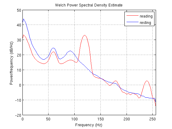
The initial step in this process was an analysis of the spectrograms and power spectral density plots collected for different trials of reading and resting. Several features seemed potential candidates to be leveraged in the algorithm. One striking difference is the presence of an intense band of activity at 120 Hz, which appears in the reading spectrogram but is absent in the resting spectrogram. Despite its stark differences, we chose not to incorporate this feature into the algorithm because we felt that it does not likely indicate a true effect occurring in the brain. Rather, its ubiquity across many of our measurements (and the fact that its frequency never wavers) led us to believe that it might be an artifact of the headset. Instead, we were more interested in the fact that the resting state appears to have more energy just above baseband, in the 10-50 Hz range. Ultimately, this was the feature we selected for in the algorithm. Because this is an effect that accumulates over the entire period of the experiment, the Power Spectral Density plot provides an excellent way to quantify these differences. As is evident in the PSD plot below, the intuitions we developed from the spectrograms are clearly confirmed to hold true for the example below. After inspecting several other trials, we decided that the 10-50 Hz frequency range selected the phenomenon we observed while excluding potential sources of noise like 60 Hz noise. Thus, we wrote a script to integrate the power in this range for the two sets of data. It then attributes the higher value to the resting state and the lower to a reading state. With the appropriately set integration limits. the algorithm correctly determined the source of the data for all of the trials we performed.

A psd comparison of reading and resting