

| << Chapter < Page | Chapter >> Page > |
An Intertemporal Choice Example
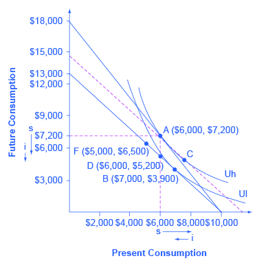
Quentin has saved up $10,000. He is thinking about spending some or all of it on a vacation in the present, and then will save the rest for another big vacation five years from now. Over those five years, he expects to earn a total 80% rate of return. [link] shows Quentin’s budget constraint and his indifference curves between present consumption and future consumption. The highest level of utility that Quentin can achieve at his original intertemporal budget constraint occurs at point A, where he is consuming $6,000, saving $4,000 for the future, and expecting with the accumulated interest to have $7,200 for future consumption (that is, $4,000 in current financial savings plus the 80% rate of return).
However, Quentin has just realized that his expected rate of return was unrealistically high. A more realistic expectation is that over five years he can earn a total return of 30%. In effect, his intertemporal budget constraint has pivoted to the left, so that his original utility-maximizing choice is no longer available. Will Quentin react to the lower rate of return by saving more, or less, or the same amount? Again, the language of substitution and income effects provides a framework for thinking about the motivations behind various choices. The dashed line, which is a graphical tool to separate the substitution and income effect, is carefully inserted with the same slope as the new opportunity set, so that it reflects the changed rate of return, but it is tangent to the original indifference curve, so that it shows no change in utility or “buying power.”
The substitution effect tells how Quentin would have altered his consumption because the lower rate of return makes future consumption relatively more expensive and present consumption relatively cheaper. The movement from the original choice A to point C shows how Quentin substitutes toward more present consumption and less future consumption in response to the lower interest rate, with no change in utility. The substitution arrows on the horizontal and vertical axes of [link] show the direction of the substitution effect motivation. The substitution effect suggests that, because of the lower interest rate, Quentin should consume more in the present and less in the future.
Quentin also has an income effect motivation. The lower rate of return shifts the budget constraint to the left, which means that Quentin’s utility or “buying power” is reduced. The income effect (assuming normal goods) encourages less of both present and future consumption. The impact of the income effect on reducing present and future consumption in this example is shown with “i” arrows on the horizontal and vertical axis of [link] .
Notification Switch
Would you like to follow the 'Principles of macroeconomics for ap® courses' conversation and receive update notifications?

|
|
|
|
|

|
|

|
|

|
|
|
|
|

|
|

|
|

|
|

|
|

|
|

|