

| << Chapter < Page | Chapter >> Page > |
Shown across the top of [link] is a stylized version of that seen in the bottom portion of [link] . The uniform weight shown on the top right leads to the bandpass filter shapes shown on the left. Note that the filters are separated in frequency by Hz.
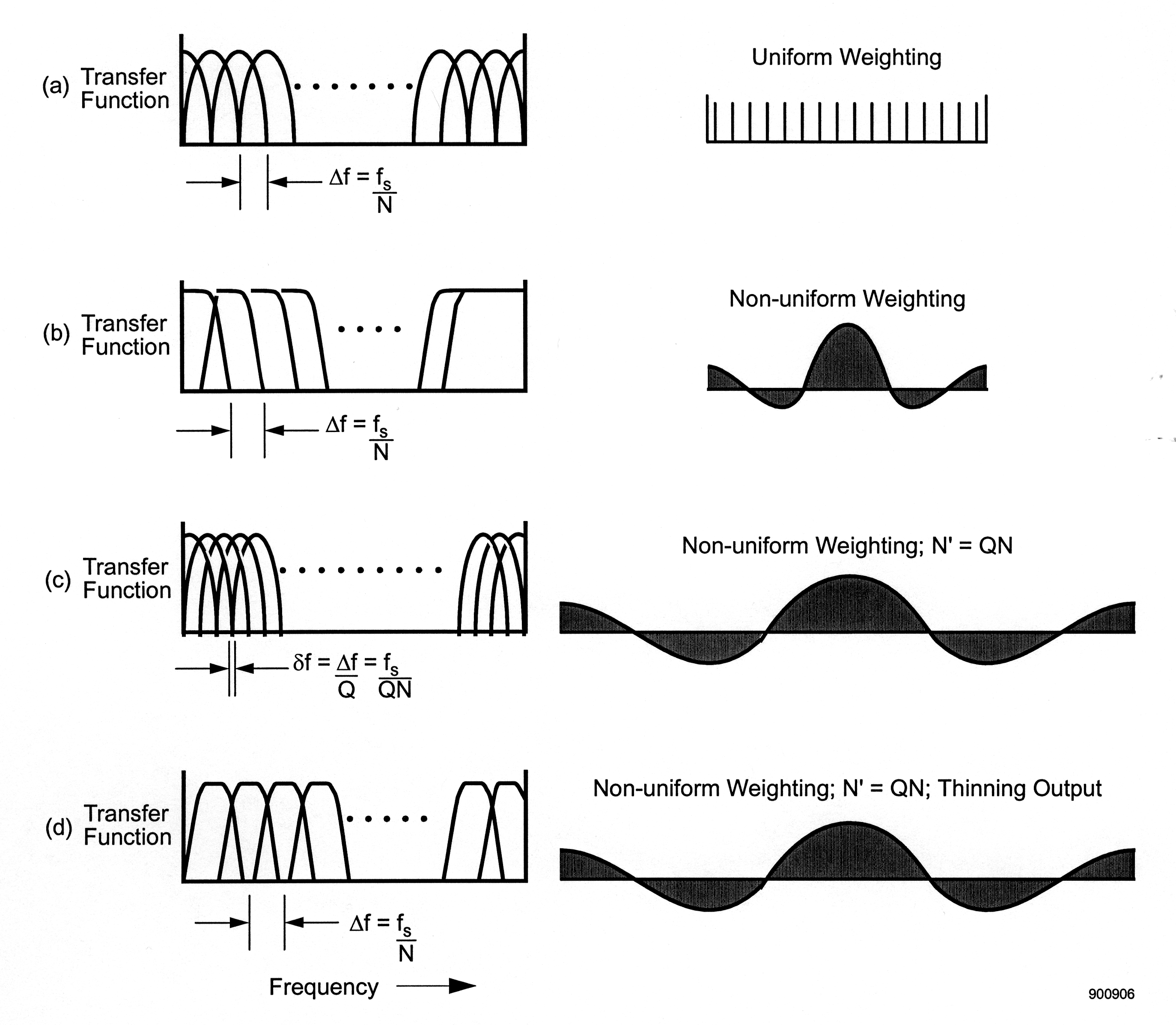
Now suppose we employ non-uniform weighting to improve the shape of the bandpass filters. As discussed in Appendix A , such non-uniform weighting can be used to attain the desired transfer function shape, but virtually always at the expense of the bandpass filter's bandwidth. In fact, to obtain the desired characteristic shown in [link] , with its flat passband, sharp skirts, and high-attenuation stopband, the minimum passband bandwidth is more than a factor of ten larger than the unweighted response. Thus the use of a non-uniform weighting, as shown on the right of [link] (b), results in the situation shown on the left side. There are still N bandpass filters, and their center frequencies are still separated by integer multiples Hz, but each filter has been widened considerably, leading to a high degree of overlap.
The first problem to deal with is not the overlap, but rather the fact that the individual bandpass filters are far wider than the original goal of about Hz. This is dealt with by returning to [link] and simply letting the delay line length, the number of weighting coefficients, and the DFT order grow until the filters are sufficiently narrowband to meet our objectives. Again using the example of the desired frequency response seen in [link] , the dimensions must grow by more than a factor of ten.
While the resulting dimensions can take on rather arbitrary values (above some minimum value) we'll assume here that the new size N' is an integer multiple of N . In particular, we assume that the delay line, and the weighting and DFT with it, are extended to the length N' where:
where Q is a positive integer. We further assume that Q is chosen to be large enough that a weighting function of length N ' can be designed to produce not only the desired shape but also a bandwidth of about Hz. The resulting situation is shown in [link] (c). The weighting function is now longer than before (by a factor of Q ). On the left we see that there are now N ' filters in the filter bank. Each one of them now has the desired nominal bandwidth of Hz, but their center frequencies are now separated by Hz instead of Hz. The overlap seen just above still exists but now there is a factor of Q more filters, a factor of Q narrower, and a factor of Q more closely spaced. Thus the positive effect of expanding the delay line dimension to is that the resulting filter bank includes the desired bandpass filters, both in bandpass characteristics and center frequencies. The negative aspects include the fact that the amount of weighting and DFT computation have gone up by a factor of Q and that there are now superfluous bandpass filters.
Suppose now that we choose to compute only every Q-th point of the DFT. The delay line is still samples long, there are still coefficients in the weighting function, and the DFT still has order , but we'll choose to only compute those output bins where m is an integer multiple of Q . This results in the situation shown in [link] (d). The same QN-point weighting function is used as immediately above. This case, with N filters of nominal bandwidth Hz and spaced Hz apart, was our objective. To achieve it, however, required expanding the dimensions of the preceding operations quite considerably.
Notification Switch
Would you like to follow the 'An introduction to the fdm-tdm digital transmultiplexer' conversation and receive update notifications?

|
|

|
|

|
|

|
|
|
|
|

|
|

|
|

|
|

|
|

|