0.17 Appendix: more on prony and pade

Iir filter design using the methods by prony and pade

Consider the filter in [link] with transfer function

We can rewrite it as

which represents the convolution $b\left(n\right)=h\left(n\right)*a\left(n\right)$ . This operation can be represented in matrix form [link] as follows,

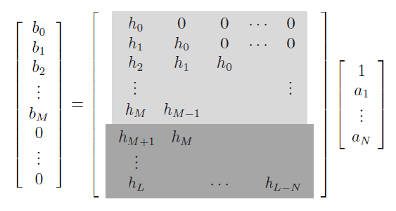
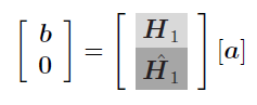
System [link] can be viewed as [link] ,

If $L=M+N$ , equations [link] and [link] describe the same square systems as equations [link] and [link] , letting $c_k$ in the former systems to become $h_k$ in the latter ones. Therefore when the number of impulse response samples to be matched is equal to $M+N$ , solving [link] for the coefficients $a_k$ and $b_k$ is equivalent to applying Pade's method to matching the first $N+M$ values of the impulse response $h\left(n\right)$ . In consequence, this method is known as Pade's method for IIR filter design [link] or simply Pade approximation method [link] , [link] . Pade's method is an interpolation algorithm; since the number of samples to be interpolated must be equal to the number of filter parameters, Pade's method is limited to very large filters, which makes it impractical.

The relationship of the above method with Prony's method can be seen by posing Prony's method in the $Z$ -domain. Consider the function $f\left(n\right)$ from [link] ,

The $Z$ -transform of $f\left(n\right)$ is given by

where $\mathcal{Z}\{·\}$ denotes the $Z$ -transform operator. By linearity of the $Z$ -transform [link] ,

Using

(the left equality is true since $f\left(n\right)=0$ for $n<0$ by assumption) in [link] we get

The numerator and denominator in [link] are two polynomials in $z^{-1}$ of degrees $N-1$ and $N$ respectively. Expanding both polynomials, equation [link] becomes

Assuming $a_0=1$ does not affect the formulation of $F\left(z\right)$ . This is equivalent to dividing both the numerator and denominator of [link] by $a_0$ . From [link] it is clear that Prony's method is in fact a particular case of the Pade approximation method described earlier in this section (with $M=N$ ). From [link] and [link] we have

Therefore, given $2N$ samples of $h\left(n\right)=f\left(n\right)$ one can solve for the parameters $c_k$ and ${\lambda }_k$ in [link] merely by applying partial fraction expansion [link] on [link] .

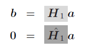
Consider the systems in [link] and [link] . If $L>M+N$ then [link] is an overdetermined system and cannot be solved exactly in general. However, it is possible to find a least squares approximation following an approach similar to the one used in the frequency domain design method from [link] . Given $L>M+N$ samples of an impulse response $h\left(n\right)$ , we rewrite ${\widehat{\mathbf{H}}}_1$ as

where

Following the same formulation of [link] , the filter coefficients $a_k$ and $b_k$ are found by solving for $\widehat{a}$ and $b$ in

where $H_1$ is an $M\times N$ matrix given by

The error analysis for these algorithms is equivalent to the one performed in [link] . In fact, both approaches (frequency sampling versus Pade's method) are quite similar. Among the common properties, both methods use an equation error criterion rather than the more useful solution error. However, it is worth to point out that in the time domain (Pade) approach, samples of the impulse response are used to make the approximation, and the method uses a linear convolution rather than the cyclic one from the frequency domain approach. Also, since the latter method uses a uniform sampling grid within the complete frequency spectrum between $\omega =0$ and $\omega =2\pi$ instead of using the first few samples of an infinitely long sequence ( $h\left(n\right)$ ), the approximation properties of the frequency domain method are superior.