0.14 L_p approximation

Infinite Impulse Response (IIR) filters are important tools in signal processing. The flexibility they offer with the use of poles and zeros allows for relatively small filters meeting specifications that would require somewhat larger FIR filters. Therefore designing IIR filters in an efficient and robust manner is an inportant problem.

This section covers the design of a number of important $l_p$ IIR problems. The methods proposed are consistent with the methods presented for FIR filters, allowing one to build up on the lessons learned from FIR design problems. The complex $l_p$ IIR problem is first presented in [link] , being an essential tool for other relevant problems. The $l_p$ frequency-dependent IIR problem is also introduced in [link] . While the frequency-dependent formulation might not be practical in itself as a filter design formulation, it is fundamental for the more relevant magnitude $l_p$ IIR filter design problem, presented in [link] .

Some complications appear when designing IIR filters, among which the intrinsic least squares solving step clearly arises from the rest. Being a nonlinear problem, special handling of this step is required. It was detemined after thorough experimentation that the quasilinearization method of Soewito presented in [link] can be employed successfully to handle this issue.

Complex and frequency-dependent $l_p$ Approximation

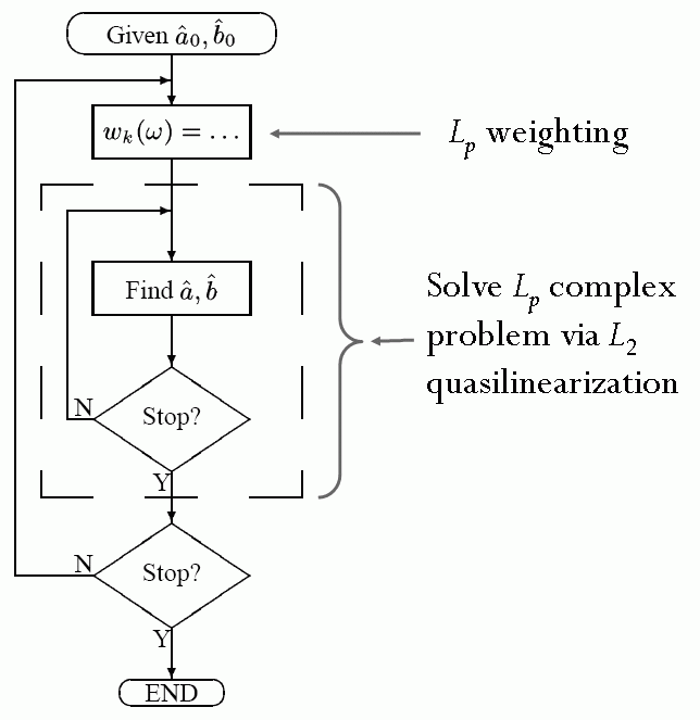
Chapter [link] introduced the problem of designing $l_p$ complex FIR filters. The complex $l_p$ IIR algorithm builds up on its FIR counterpart by introducing a nested structure that internally solves for an $l_2$ complex IIR problem. [link] illustrates this procedure in more detail. This method was first presented in [link] .

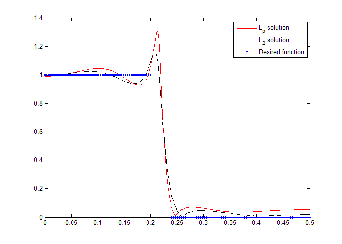
Compared to its FIR counterpart, the IIR method only replaces the weighted linear least squares problem for Soewito's quasilinearization algorithm. While this nesting approach might suggest an increase in computational expense, it was found in practice that after the initial $l_2$ iteration, in general the $l_p$ iterations only require from one to only a few internal weighted $l_2$ quasilinearization iterations, thus maintaining the algorithm efficiency. Figures [link] through [link] present results for a design example using a length-5 IIR filter with $p=100$ and transition edge frequencies of 0.2 and 0.24 (in normalized frequency).

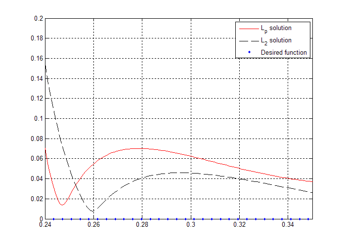
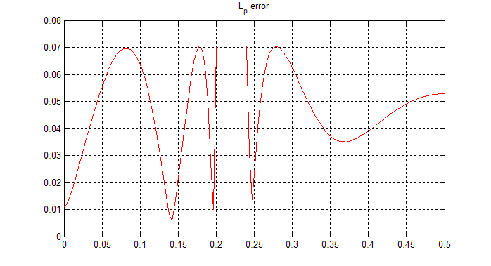
[link] compares the $l_2$ and $l_p$ results and includes the desired frequency samples. Note that no transition band was specified. [link] illustrates the effect of increasing $p$ . The largest error for the $l_2$ solution is located at the transition band edges. As $p$ increases the algorithm weights the larger errors heavier; as a result the largest errors tend to decrease. In this case the magnitude of the frequency response went from 0.155 at the stopband edge (in the $l_2$ case) to 0.07 (for the $l_p$ design). [link] shows the error function for the $l_p$ design, illustrating the quasiequiripple behavior for large values of $p$ .

Another fact worth noting from [link] is the increase in the peak in the right hand side of the passband edge (around $f=0.22$ ). The $l_p$ solution increased the amplitude of this peak with respect to the corresponding $l_2$ solution. This is to be expected, since this peak occurs at frequencies not included in the specifications, and since the $l_p$ algorithm will move poles and zeros around in order to meet find the optimal $l_p$ solution (based on the frequencies included for the filter derivation). The addition of a specified transition band function (such as a spline) would allow for control of this effect, depending on the user's preferences.