0.11 Lecture 12:interconnected systems and feedback

Lecture #12:

INTERCONNECTED SYSTEMS AND FEEDBACK

Motivation:

• Signals normally pass through interconnections of subsystems.

• Feedback is widely used in both man-made and natural systems to enhance performance.

• Feedback provides an opportunity to use and to integrate material we have learned (Laplace transform, frequency response, step response) in an important application area.

• Stability is an important issue with feedback systems

• Unstable systems can be stabilized with feedback

Outline:

• Interconnection of systems
• Simple feedback system — Black’s formula
• Effect of feedback on system performance

• Review properties of feedback
• Dynamic performance of feedback systems
• BIBO stability
• Roots of second-order and third-order polynomials
• Root locus plots of position control systems
• Stabilization of unstable systems
• Conclusion

I. INTERCONNECTION OF SYSTEMS

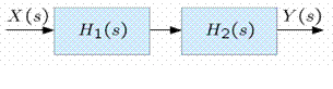
Systems are interconnections of sub-systems. For example, consider the cascade of LTI systems shown below.

The presumption in such a cascade is that H1(s) and H2(s) do not change when the two systems are connected.

1/ Cascade of a lowpass and a highpass filter

Suppose $H_1(s)$ and $H_2(s)$ have the following form.

$H_1(s)=\frac{Y_1(s)}{X_1(s)}=\frac{\frac{1}{R_1{C}_1}}{s+\frac{1}{R_1{C}_1}}$

$H_2(s)=\frac{Y_2(s)}{X_2(s)}=\frac{s}{s+\frac{1}{R_2{C}_2}}$

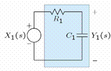
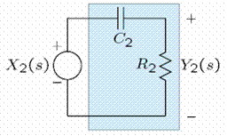
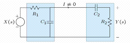
2/ Loading

Now cascade $H_1(s)$ and $H_2(s)$ .

l

$H_1(s)=\frac{\frac{1}{R_1{C}_1}s}{s^2+s\left[\frac{1}{R_1{C}_1}+\frac{1}{R_2{C}_2}+\frac{1}{R_2{C}_1}\right]+\frac{1}{R_1{R}_2{C}_1{C}_2}}$

Note that

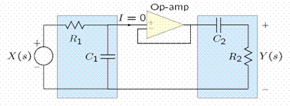
3/ Isolation

With the use of an op-amp, the two systems can be isolated from each other or buffered so that the system function is the product of the individual system functions.

Note that

4/ Conclusion

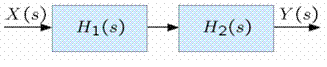
When we draw block diagrams of the form

we assume that the individual systems are buffered or that the loading of system 1 by system 2 is taken into account in $H_1(s)$

II. FEEDBACK EXAMPLES

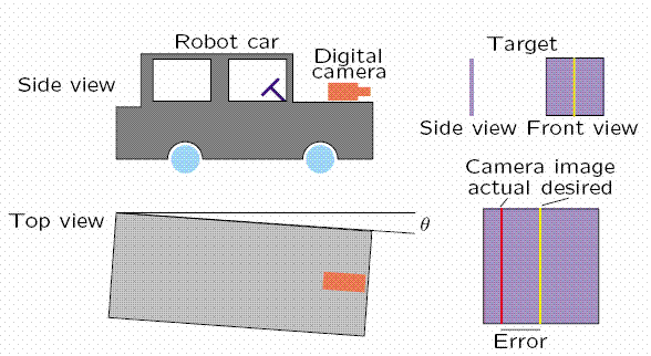
1/ Man-made system — robot car

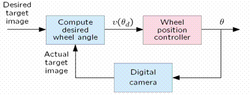
2/ Robot car block diagram

To drive the robot car to the target we use the camera to compare the measured target position with the desired target position. The difference is an error signal whose value is used to change the wheel position. Therefore, the output variable, the angle of the wheels, is fed back to the input to control the new output variable.

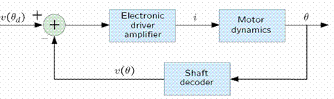
3/ Wheel position controller block diagram

The wheel controller system is itself a feedback system. A voltage proportional to the angular position of the motor shaft is subtracted from the desired value and the difference signal is used to drive the motor.

4/ Physiological control systems examples

Voluntary everyday activities

• Driving a car
• Filling a glass with water

Involuntary everyday occurrences

• Pupil reflex
• Blood glucose control
• Spinal reflex

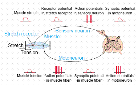
5/ Spinal reflex

Tapping the patella stretches muscle receptors that, through a neural feedback system, results in muscle contraction. This reflex is used in the maintenance of posture.