0.10 Lecture 11:sinusoidal steady-state (sss) or frequency response  (Page 5/5)

$Z(s)=G\frac{\left[\frac{s}{{\omega }_0}\right]}{{\left[\frac{s}{{\omega }_0}\right]}^2+\frac{1}{Q}\left[\frac{s}{{\omega }_0}\right]+1}$

Where

$\begin{array}{}{\omega }_0=\frac{1}{(\text{LC}{)}^{1/2}}\begin{array}{cc}& \end{array}(\text{Undamped}\begin{array}{cc}& \end{array}\text{resonant}\begin{array}{cc}& \end{array}\text{frequency})\\ Q=R{\left[\frac{C}{L}\right]}^{1/2}\begin{array}{cc}& \end{array}(\text{Quality}\begin{array}{cc}& \end{array}\text{of}\begin{array}{cc}& \end{array}\text{resonance})\\ G={\left[\frac{C}{L}\right]}^{1/2}\begin{array}{cc}& \end{array}(\text{Gain}\begin{array}{cc}& \end{array}\text{cons}\text{tan}t)\end{array}$

4/ Normalized resonance function

$Z(s)=G\frac{\left[\frac{s}{{\omega }_0}\right]}{{\left[\frac{s}{{\omega }_0}\right]}^2+\frac{1}{Q}\left[\frac{s}{{\omega }_0}\right]+1}=\text{GR}\left[\frac{s}{{\omega }_0}\right]$

where

$R(s)=\frac{s}{s^2+\frac{1}{Q}s+1}$

Therefore, Z(s) and R(s) are the same except for differences in scale. R(s), which is a universal second-order function, depends on only one parameter, Q.

5/ Properties of R(s)

R(s) has a zero at s = 0 and poles at

$\{\begin{array}{c}{p}_1=-\left[\frac{1}{\mathrm{2Q}}\right]+{\left[{\left[\frac{1}{\mathrm{2Q}}\right]}^2-1\right]}^{1/2}\\ p_2=-\left[\frac{1}{\mathrm{2Q}}\right]-{\left[{\left[\frac{1}{\mathrm{2Q}}\right]}^2-1\right]}^{1/2}\end{array}$

As Q is varied the poles trace out a trajectory in the s-plane called a root-locus plot.

• For 0<Q<<1/2, the poles are near 0, and −1/Q.
• For Q ≤ 1/2, the poles are on the real axis.
• For Q = 1/2, both poles are at −1.
• For Q>1/2, the poles are complex and the locus is circular.

6/ High-Q filter

Recall that for the parallel RLC circuit

$Q=R{\left[\frac{C}{L}\right]}^{1/2}$

When R is arbitrarily large, Q becomes arbitrarily large and we call the network a high-Q system. Note also that in this limit, the current through the resistance becomes arbitrarily small, and it can be shown that the network dissipates relatively little energy.

We shall examine the frequency response of the network in this high-Q limit.

7/ Low-frequency asymptote for the high-Q system

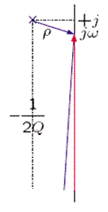
R(s) has one zero and two complex conjugate poles, i.e.,

$R(s)=\frac{s}{(s-p)(s-p^{})}$

A vector diagram is used to interpret the behavior of the system at low frequencies.

At low frequencies, ω<<1, and the system function evaluated at s = jω is

$R(\mathrm{j\omega })\approx \frac{\mathrm{j\omega }}{(-j)(+j)}=\mathrm{j\omega }$

8/ High-frequency asymptote for the high-Q system

We can use a vector diagram to interpret the behavior of the system at high frequencies as follows.

At high frequencies, ω _ 1, and the system function evaluated at s = jω is

9/ Behavior of the high-Q system near the resonant frequency

For ω ≈ 1

$R(\mathrm{j\omega })\approx \frac{\mathrm{j1}}{(\rho )(\mathrm{j2})}=\frac{1}{\mathrm{2\rho }}$

For w = 1

$\mid R(\mathrm{j1})\mid \approx \frac{1}{2(1/(\mathrm{2Q}))}=Q\begin{array}{cc}& \end{array}\text{and}\begin{array}{cc}& \end{array}\angle R(\mathrm{j1})\approx 0$

For $w=1\pm \frac{1}{\mathrm{2Q}}$

$\begin{array}{}\mid R\left[j\left[1\pm \frac{1}{\mathrm{2Q}}\right]\right]\mid \approx \frac{1}{2(1/(\mathrm{2Q}))2^{1/2}}=\frac{Q}{2^{1/2}}\\ \angle R\left[j\left[1\pm \frac{1}{\mathrm{2Q}}\right]\right]\approx \mp \frac{\pi }{4}\end{array}$

10/ Frequency response of the high-Q system

The frequency response, R(jω), is shown in linear coordinates near the resonant frequency (ω = 1). This bandpass filter passes frequencies maximally in a bandwidth BW near the resonant frequency and attenuates frequencies outside that band.

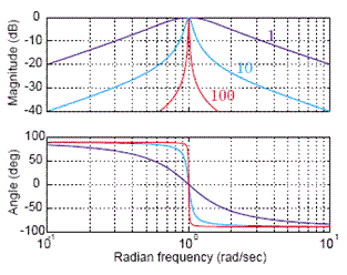
R(jω) is shown in logarithmic coordinates for Q = 10.

The low-frequency asymptote has a magnitude slope of +20 dB/decade and an angle of +90o and the high-frequency asymptote slope is −20 dB/decade and an angle of −90o

11/ Constant-Q filters

We plot the frequency response for bandpass filters with the same value of Q but different resonant frequencies.

For

$Z(s)=G\frac{\left[\frac{s}{{\omega }_0}\right]}{{\left[\frac{s}{{\omega }_0}\right]}^2+\frac{1}{Q}\left[\frac{s}{{\omega }_0}\right]+1}$

we plot frequency responses for G = 1, Q = 10, ${\omega }_0=1$ , ${\text{10}}^{1/2}$ , 10, and ${\text{10}}^{3/2}$ ,

12/ Constant- ωo filters

We plot the frequency response for bandpass filters with the same value of ωo but different values of Q.

For

$Z(s)=G\frac{\left[\frac{s}{{\omega }_0}\right]}{{\left[\frac{s}{{\omega }_0}\right]}^2+\frac{1}{Q}\left[\frac{s}{{\omega }_0}\right]+1}$

we plot frequency responses for G = 1/Q, ω = 1. The parameter is Q = 1, 10, and 100.

Two-minute miniquiz problem

Problem 7-1 Frequency response of a resonant system

Given

$H(s)=\text{10}\frac{s}{(s+1{)}^2+\text{100}}$

Determine (approximately)

a) the resonant frequency,

b) the bandwidth,

c) |H(jω)| at the resonant frequency.

Solution

The system function has a zero at s = 0 and poles at s = −1 ± j10. Near resonance the vector diagram looks as follows

a) The resonant frequency is ${\omega }_0\approx \text{10}\text{rad}/s$ .

b) From a vector interpretation, the frequency response has 3 dB points at 9 and 11 rad/s. Hence, the bandwidth is 2 rad/s.

c) From a vector interpretation,

$H(j\text{10})\approx \text{10}\frac{j\text{10}}{(1)(j\text{20})}=5$

13/ Use of bpf for extraction of narrow-band signals in wideband noise

A resonant circuit acting as a narrow-band or bandpass filter (BPF) can be used to extract a narrow-band signal from wideband noise. The resonant frequency of the filter is set to equal

the center frequency of the signal. The value of Q is chosen to determine the desired amount of attenuation of the wide-band noise.

VIII. SECOND-ORDER NOTCH FILTERS

1/ Notch filter — system function and pole-zero diagram

A second-order notch filter has the form shown below.

$H(s)=\frac{{\left[\frac{s}{{\omega }_0}\right]}^2+1}{{\left[\frac{s}{{\omega }_0}\right]}^2+\frac{1}{Q}{\left[\frac{s}{{\omega }_0}\right]}^2+1}$

2/ Notch filter — frequency response

$H(\mathrm{j\omega })=\frac{1-{\left[\frac{\omega }{{\omega }_0}\right]}^2}{1-{\left[\frac{\omega }{{\omega }_0}\right]}^2+j\frac{1}{Q}\left[\frac{\omega }{{\omega }_0}\right]}$

The notch filter has a frequency response

3/ Use of notch filter to attenuate narrow-band noise in a wide-band signal

A notch filter (NF) can be used to attenuate a narrow-band noise in a wide-band signal. The resonant frequency of the filter is set to equal the center frequency of the noise. The value of Q is chosen to determine the desired amount of attenuation of the narrow-band noise. In the example shown, a LPF and HPF can also be used if there is sufficient frequency separation between desirable and undesirable components of the signals.

IX. CONCLUSIONS

The frequency response

• is the system function evaluated along the jω-axis,
• has a simple geometric interpretation in the s-plane,
• describes the filtering of an input sinusoid to an LTI system,
• has asymptotes that are easily sketched in a Bode diagram when the poles and zeros lie on the negative real axis.

Filters have been illustrated to perform a variety of important signal processing tasks. The filters we have introduced are

• lowpass and highpass filters both first-order and higher order,
• bandpass filters consisting of resonant systems,
• notch filters.