These are determined from N initial conditions which must be specified. These conditions result in a set of N algebraic equations that need to be solved to obtain the initial conditions. We shall find another, and simpler, method to determine these coefficients later.
2/ Steady-state
Assume the particular solution is not zero. Then the particular solution dominates after some time, if the homogeneous solution decays more rapidly than does the particular solution. When this occurs, we call the resulting particular solution the steady-state response. Steady-state occurs if each term in the homogeneous solution decays more rapidly than the particular solution. Thus, steady-state occurs if
Thus
which implies that
Thus, steady-state occurs when
for all
provided the particular solution is not zero. The conditions for steady state are depicted in the complex s plane below.
The particular solution dominates for s in the shaded region, and the total solution equals the steady-state solution i.e.,
For which conditions is the particular solution zero? Suppose
The particular solution dominates for s in the shaded region, and the total solution equals the steady-state solution except when s = 1 because at this value i.e.,
so that the particular solution is zero and steady -state does not occur.
IX. LINEAR DIFFERENCE EQUATIONS ARISE IN MANY DIFFERENT CONTEXTS
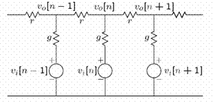
1/ Electric ladder network
r is the series resistance and g is the shunt conductance.
KCL at the central node yields
which yields the linear difference equation
2/ Interest and accumulation
Let us consider a simple model of the accumulation of wealth through savings. At the end of year n you deposit x[n] dollars in the bank which pays an annual interest of r. Your accumulation at the end of year n is y[n]dollars. Therefore,
We can rewrite this equation as
y[n+1] − (1+r)y[n]= x[n]
This difference equation can be realized in a block diagram as shown below.
D is a unit delay unit.
3/ Discretized CT system
An important application of DT systems is a numerical simulation of a CT system. For example, consider the CT lowpass filter shown below.
The differential equation is
To solve this equation numerically in a computer, the CT signals are discretized and the derivative is approximated.
To discretize the signals, we can define DT signals as samples of CT signals, i.e.,
and
The derivative can be approximated as follows
Therefore, we can approximate the differential equation as
which can be written as
Let
= T/(RC). Then the difference equation is
This equation can be solved iteratively for a given input and initial condition. Assume that
and that
then
Questions & Answers
differentiate between demand and supply
giving examples
In economics, a perfect market refers to a theoretical construct where all participants have perfect information, goods are homogenous, there are no barriers to entry or exit, and prices are determined solely by supply and demand. It's an idealized model used for analysis,
When MP₁ becomes negative, TP start to decline.
Extuples Suppose that the short-run production function of certain cut-flower firm is given by: Q=4KL-0.6K2 - 0.112 •
Where is quantity of cut flower produced, I is labour input and K is fixed capital input (K-5). Determine the average product of lab
Kelo
Extuples Suppose that the short-run production function of certain cut-flower firm is given by: Q=4KL-0.6K2 - 0.112 •
Where is quantity of cut flower produced, I is labour input and K is fixed capital input (K-5). Determine the average product of labour (APL) and marginal product of labour (MPL)
Quantity demanded refers to the specific amount of a good or service that consumers are willing and able to purchase at a give price and within a specific time period. Demand, on the other hand, is a broader concept that encompasses the entire relationship between price and quantity demanded
Ezea
ok
Shukri
how do you save a country economic situation when it's falling apart
Economic growth as an increase in the production and consumption of goods and services within an economy.but
Economic development as a broader concept that encompasses not only economic growth but also social & human well being.
Shukri
production function means
Jabir
What do you think is more important to focus on when considering inequality ?
sir...I just want to ask one question... Define the term contract curve? if you are free please help me to find this answer 🙏
Asui
it is a curve that we get after connecting the pareto optimal combinations of two consumers after their mutually beneficial trade offs
Awais
thank you so much 👍 sir
Asui
In economics, the contract curve refers to the set of points in an Edgeworth box diagram where both parties involved in a trade cannot be made better off without making one of them worse off. It represents the Pareto efficient allocations of goods between two individuals or entities, where neither p
Cornelius
In economics, the contract curve refers to the set of points in an Edgeworth box diagram where both parties involved in a trade cannot be made better off without making one of them worse off. It represents the Pareto efficient allocations of goods between two individuals or entities,
Cornelius
Suppose a consumer consuming two commodities X and Y has
The following utility function u=X0.4 Y0.6. If the price of the X and Y are 2 and 3 respectively and income Constraint is birr 50.
A,Calculate quantities of x and y which maximize utility.
B,Calculate value of Lagrange multiplier.
C,Calculate quantities of X and Y consumed with a given price.
D,alculate optimum level of output .
the market for lemon has 10 potential consumers, each having an individual demand curve p=101-10Qi, where p is price in dollar's per cup and Qi is the number of cups demanded per week by the i th consumer.Find the market demand curve using algebra. Draw an individual demand curve and the market dema
suppose the production function is given by ( L, K)=L¼K¾.assuming capital is fixed find APL and MPL. consider the following short run production function:Q=6L²-0.4L³ a) find the value of L that maximizes output b)find the value of L that maximizes marginal product