|
|
Published: September 20, 2005
By Richard G. Baldwin
Java Programming, Notes # 2350
DSP and adaptive filtering
With the decrease in cost and the increase in speed of digital devices, Digital Signal Processing (DSP) is showing up in everything from cell phones to hearing aids to rock concerts. Many applications of DSP are static. That is, the characteristics of the digital processor don't change with time or circumstances. However, a particularly interesting branch of DSP is adaptive filtering. This is a situation where the characteristics of the digital processor change with time, circumstances, or both.
First in a series
This is the first lesson in a series designed to teach you about adaptive filtering in Java. This lesson will introduce you to the topic by showing you how to write a Java program to solve a relatively simple time-adaptive filtering problem for which the correct solution is well known in advance. This will make it possible to check the adaptive solution against the known correct solution.
An adaptive whitening filter
The next lesson will show you how to write an adaptive whitening filter program in Java, which is conceptually more difficult than the filter that I will explain in this lesson. The next lesson will also show you how to use the whitening filter to extract wide band signal from a channel in which the signal is corrupted by one or more components of narrow band noise.
More general adaptive filtering considerations
Following that, the lessons in the series will become somewhat more general. I plan to publish lessons that explain and provide examples for the four common scenarios in which adaptive filtering is used:
Somewhere along the way I will probably also publish a lesson that explains and illustrates the difference between least mean square (LMS) and recursive least squares (RLS) adaptive algorithms.
Viewing tip
You may find it useful to open another copy of this lesson in a separate browser window. That will make it easier for you to scroll back and forth among the different figures and listings while you are reading about them.
Supplementary material
I recommend that you also study the other lessons in my extensive collection of online Java tutorials. You will find those lessons published at Gamelan.com. However, as of the date of this writing, Gamelan doesn't maintain a consolidated index of my Java tutorial lessons, and sometimes they are difficult to locate there. You will find a consolidated index at www.DickBaldwin.com.
A time-delay filter with a flat amplitude response
The program that I will present and explain in this lesson illustrates an aspect of adaptive filtering for which the correct solution is already well known. The program adaptively designs a time-delay filter with a flat amplitude response and a linear phase response in the frequency domain.
A straightforward but useful scenario for learning
Although this is a relatively straightforward scenario, it is also a useful scenario for learning purposes. To begin with, the program illustrates the use of a least mean square (LMS) adaptive algorithm in a relatively simple setting, making it easy to understand what the algorithm is doing. In addition, the program teaches you about the use of digital delay lines, a topic with which you may not yet be familiar. Beyond that, it is easy to confirm that the adaptive solution matches the known correct solution.
User experimentation is encouraged
When running this program, the user provides several parameters that have an impact on the adaptive process. This allows the user to experiment with the adaptive process comparing results for different input parameters.
Two channels of input data
Two sampled time series, chanA and chanB, are presented to the adaptive processing system. Each time series consists of the same wide band signal plus white noise that is uncorrelated between the two channels.
A time shift between the two channels
On the basis of user input, the signal in chanB can be delayed or advanced by up to six samples relative to the signal in chanA. In other words, the time base for chanB can be shifted in either direction causing chanB to lead chanA in time, or causing chanB to lag chanA in time.
(Also, for a trivial case, the time shift between the two channels can be set to zero.)
Filtering chanA
A nine-point convolution operator is developed adaptively and applied to chanA. The purpose of the adaptive process is to cause the filtered output to be in time registration with chanB.
(Because the coefficient values in the convolution operator change with time, the convolution process also changes with time.)
How do you measure success?
When the adaptive process converges successfully, the time series produced by applying the convolution operator to chanA matches the signal on chanB.
It is already well known that the correct solution to this problem is a finite impulse response (FIR) convolution filter in which one coefficient has a value of 1 and all the other coefficients have a value of 0. The location of the coefficient having the value of 1 is such as to cause the result of filtering chanA to be either advanced or delayed in time by a number of samples that causes it to be in time registration with chanB.
It is also already well known that the Fourier transform of the filter described above will have a flat amplitude response and a linear phase response.
If the adaptive process converges to this result, it is successful.
User inputs
The user provides the following information as command line parameters:
The first example was run using default parameters. This produced the following output on the command line screen. (Note that a line break was manually entered into the first line to force it to fit into this narrow publication format.)
Usage: java Adapt01 timeShift feedbackGain
noiseLevel numberIterations
Negative timeShift is delay
Using -4 sample shift by default
Using 0.001 feedbackGain by default
noiseLevel is a decimal fraction
Using 0.0 by default
numberIterations is an int
Using 100 by default
Graphic output
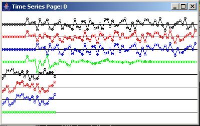
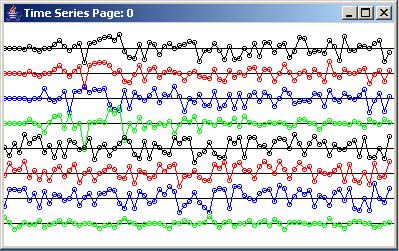
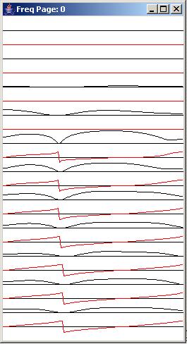
Figure 1 shows the first of three graphic outputs that are produced by this program. (The other two graphic outputs are shown later in Figure 2.)
The following four time series are plotted in color in Figure 1 showing the convergence (or lack thereof) of the adaptive algorithm:
|
|
Figure 1
Traces wrap around and down
When the top four traces reach the right end of the plotting area in Figure 1, they wrap around and down resulting in four new traces further down the page. Thus, the bottom four traces in Figure 1 are the continuation of the right end of the top four traces.
Was the adaptive process successful?
If the adaptive process is successful for this problem, the green (error) trace should go to zero, and the red (filter output) trace should match the blue (target) trace. As you can see, the adaptive process converges to this solution about half way across the top four traces in Figure 1. Thus, the adaptive process was successful. I will have more to say about Figure 1 later when I explain the code.
Impulse response plots
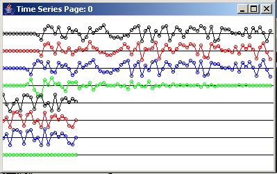
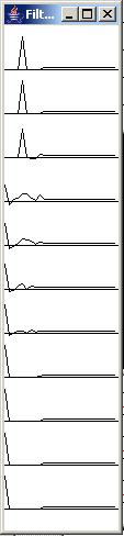
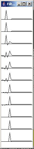
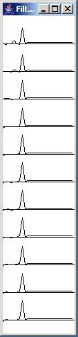
The second of the three graphic outputs produced by this program is shown in the left column of Figure 2.
The impulse response of the adaptive convolution filter at the beginning and at the end of every tenth iteration is shown in the left column of Figure 2. Thus, the changes in the shape of the impulse response can be viewed from the beginning to the end of the adaptive process.
The progressive stages of the impulse response are shown from top to bottom in the left column in Figure 2.
 |
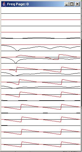 |
Figure 2
(Note that the actual impulse response consists of the values to the left of the flat raised portion of the plots in the left column of Figure 2. The minimum allowable width of an AWT Frame object in Java running under WinXP is 112 pixels, and the length of the impulse response was insufficient to fill that width. Therefore, I plotted the flat raised portion to the right of the impulse response to flag the portion of the plots that is not part of the impulse response.)
Initial impulse response at the top
The filter is initialized with a single coefficient value of 1 at the center and 0 for all of the other eight coefficient values. The correct solution is a single coefficient value of 1 at a location in the convolution filter that matches the time shift between chanA and the target, chanB. For the case shown in Figure 2, the target was delayed by four samples relative to chanA.
The peak shifts to the left
As you can see from Figure 2, the impulse response begins at the top with a value of 1 in the center and values of 0 elsewhere. As the adaptive process progresses down the page, the peak value in the impulse response progresses from the center of the impulse response to the correct location at the left end. In other words, the impulse response modifies itself such that after about 70 iterations (the eighth impulse response plot), it has a value of 1 at the left end and zeros elsewhere.
The frequency response
The third graphic output produced by this program is shown in the right column of Figure 2.
The frequency response of the convolution filter at the beginning and at the end of every tenth iteration is computed and displayed in the right column of Figure 2. Both the amplitude response and the phase response of the filter are displayed, with the amplitude response being plotted above the phase response in the right column of Figure 2. The frequency-domain plots in the right column extend from zero frequency on the left to the Nyquist folding frequency, (which is one-half the sampling frequency), on the right.
Frequency response on the right corresponds to impulse response on the left
Each pair of plots in the right column immediately to the right of a single impulse response in the left column consists of the amplitude and phase responses of the corresponding impulse response. The amplitude response is plotted in black and the phase response is plotted in red below the amplitude response.
Frequency response starts out flat
At the beginning (at the top), the impulse response consists of a single impulse in the center of the convolution filter.
(The center of the convolution filter is defined as the zero time origin for purposes of computing the phase response.)
At that point in the adaptive process, both the amplitude response and the phase response of the convolution filter are flat across the entire frequency spectrum.
Deviations appear by the twentieth iteration
By the third impulse response going down the page (twenty adaptive iterations), the impulse response is no longer represented by a single impulse, and some deviation from flatness is apparent in the corresponding amplitude response.
By the fourth impulse response (thirty adaptive iterations), the shape of the impulse response has changed considerably and quite a lot of activity is apparent in the corresponding amplitude response and phase response.
An adaptive solution in 90 iterations
By the eighth impulse response (70 iterations), the impulse response has become a single time-shifted impulse, the amplitude response has returned to being flat across the frequency spectrum, and the phase response has taken on a saw tooth character.
This is the correct solution as described above.
A flat amplitude response
The fact that the impulse response is once again a single impulse means that the amplitude response of the convolution filter is flat across the entire frequency spectrum.
The new location (relative to the zero time origin) of the single impulse in the convolution filter causes the output of the filter to be shifted in time relative to its input. As evidenced in Figure 1, this causes the convolution filter output (red) to be in time registration with the target (blue). At that point, the error (green) has converged to zero.
A linear phase response
A convolution operator that produces a simple time shift is represented in the frequency domain by a flat amplitude response and a linear relationship between phase and frequency. In other words, the phase is a straight line that goes through the zero frequency origin. The slope of the line indicates the direction of the time shift. The magnitude of the slope indicates the amount of the time shift.
Because the phase response is plotted in the range from -180 degrees to +180 degrees, and wraps around whenever it exceeds either of those limits, a linear phase shift has a saw tooth appearance when plotted as shown near the bottom of Figure 2.
Testing
This program was tested using J2SE 5.0 and WinXP. J2SE 5.0 or later is required.
The program named Adapt01
I will discuss and explain this program in fragments. A complete listing of the program is provided in Listing 32 near the end of the lesson.
The beginning of the class and the beginning of the main method is shown in Listing 1.
class Adapt01{
public static void main(String[] args){
//Default values
int timeShift = -4;
double feedbackGain = 0.001;
double noiseLevel = 0.0;
int numberIterations = 100;
if(args.length != 4){
System.out.println(
"Usage: java Adapt01 " +
"timeShift feedbackGain " +
"noiseLevel numberIterations");
System.out.println(
"Negative timeShift is delay");
System.out.println(
"Using -4 sample shift by default");
System.out.println(
"Using 0.001 feedbackGain by default");
System.out.println(
"noiseLevel is a decimal fraction");
System.out.println("Using 0.0 by default");
System.out.println(
"numberIterations is an int");
System.out.println("Using 100 by default");
}else{//Command line params were provided.
//Convert String to int
timeShift = Integer.parseInt(args[0]);
System.out.println(
"timeShift: " + timeShift);
//Convert String to double
feedbackGain = Double.parseDouble(args[1]);
System.out.println(
"feedbackGain: " + feedbackGain);
//Convert String to double
noiseLevel = Double.parseDouble(args[2]);
System.out.println(
"noiseLevel: " + noiseLevel);
//Convert String to int
numberIterations =
Integer.parseInt(args[3]);
System.out.println(
"numberIterations: " + numberIterations);
}//end else
if(abs(timeShift) > 6){
System.out.println(
"Time shift magnitude > 6 not allowed.");
System.out.println("Terminating");
System.exit(0);
}//end if |
The code in the main method in Listing 1 deals with the command line parameters. If the user enters command line parameters, those parameters are used in the adaptive process. If the user doesn't enter command line parameters, a set of default parameters are used in the adaptive process.
The code in Listing 1 is completely straightforward and shouldn't require explanation.
Perform the adaptive process
The code in Listing 2 instantiates an object of the Adapt01 class and invokes the process method to cause the adaptive process to be performed. As described above, the parameters passed to the process method are either provided by the user as command line parameters, or provided by the program by default if the user doesn't enter command line parameters.
new Adapt01().process(timeShift, feedbackGain, noiseLevel, numberIterations); }//end main |
Listing 2 also signals the end of the main method.
The parameters for Figure 1 and Figure 2
The case that produced the output shown in Figure 1 and Figure 2 was run without entering command line parameters. Hence, the adaptive process was executed using the following default parameters, which were displayed by the code in the main method:
Using -4 sample shift by default
Using 0.001 feedbackGain by default
noiseLevel is a decimal fraction
Using 0.0 by default
numberIterations is an int
Using 100 by default
The process method of the Adapt01 class
The process method of the Adapt01 class begins in Listing 3. The code in Listing 3 begins by declaring and populating a nine-element array of type double containing the initial convolution filter. This is the filter that is shown by the impulse response at the top of the left column in Figure 2. The contents of this array will be adaptively modified as the program executes.
void process(int timeShift,
double feedbackGain,
double noiseLevel,
int numberIterations){
//Create the initial convolution filter.
double[] filter = {0,0,0,0,1,0,0,0,0};
//Create array objects that will be used as
// delay lines.
double[] rawData = new double[13];
double[] chanA = new double[9];
double[] chanB = new double[9]; |
Create three tapped delay line objects
Then the code in Listing 3 declares three array objects, which will be used as tapped delay lines for the rawData, chanA, and chanB.
A delay line is similar to a queue. For example, think of a short section of hose that is full of colored marbles. When you insert a new marble in one end, a marble gets pushed out and discarded from the other end. Now think of cutting a series of small holes along the hose through which you can see the color of the marble next to each hole. You can think of these holes as taps from which you can extract the color of the marbles as they progress past the holes.
Each of the delay lines in this program is implemented using an array object. Data enters the delay line at the topmost element and moves to the next lower element once during each iteration. The data value that is in element 0 during a particular iteration is discarded and replaced by the value from element 1 during the next iteration.
The ability for the code to access any individual element provides taps by which the contents at any stage in the delay line can be retrieved by the code.
Instantiate a plotting object for time series data
The code in listing 4 instantiates an object of the class named PlotALot05, which provides the ability to plot the time series data in the format shown in Figure 1.
PlotALot05 plotObj = new PlotALot05( "Time Series",398,250,25,5,4,4); |
The class named PlotALot05 is a simple extension of the class named PlotALot04, which I explained in the lesson titled Plotting Large Quantities of Data using Java. I will refer you to that lesson for a general explanation of the class.
(The source code for the class named PlotALot05 is provided in Listing 33 near the end of this lesson.)
Output on the command-line screen
The parameters passed to the constructor for the class caused the constructor to display the following information about the plotting object on the command line screen.
Title: Time Series
Frame width: 398
Frame height: 250
Page width: 390
Page height: 223
Trace spacing: 25
Sample spacing: 5
Traces per page: 8
Samples per page: 156
Instantiate a plotting object for frequency response data
The code in Listing 5 instantiates a plotting object for two channels of frequency response data. One channel is used to plot the amplitude response in db and the other channel is used to plot the phase on a scale that extends from -180 degrees to +180 degrees.
PlotALot03 freqPlotObj =
new PlotALot03("Freq",264,487,20,2,0,0); |
The class named PlotALot03 is one of the classes that I explained in the earlier lesson titled Plotting Large Quantities of Data using Java. (I will refer you back to that lesson for a copy of the source code for this class.) The parameters that describe this plotting object are given below.
Title: Freq
Frame width: 264
Frame height: 487
Page width: 256
Page height: 460
Trace spacing: 20
Sample spacing: 2
Traces per page: 22
Samples per page: 1408
Instantiate a plotting object for the impulse response data
The code in Listing 6 instantiates a plotting object to display the impulse response of the convolution filter at intervals during the adaptive process. I explained the class named PlotALot01 in the earlier lesson titled Plotting Large Quantities of Data using Java. (Once again, I will refer you back to that lesson for a copy of the source code for this class.)
PlotALot01 filterPlotObj = new PlotALot01( "Filter",(filter.length * 4) + 8, 487,40,4,0,0); |
The actual plotting object parameters
The actual parameters that describe this plotting object are:
Title: Filter
Frame width: 112
Frame height: 487
Page width: 104
Page height: 460
Trace spacing: 40
Sample spacing: 4
Traces per page: 11
Samples per page: 286
The Frame width is different
Note that the actual Frame width of 112 is different from the specified Frame width of 44 in Listing 6. This is because the minimum allowable width for an AWT Frame object is 112 pixels under WinXP regardless of the specified width.
(As described below, this code is very specific to the WinXP operating system for correct plotting of the impulse response data.)
Because the actual Frame width doesn't match the specified Frame width, the code in Listing 6 won't cause the plotting process to synchronize properly and to plot a single impulse response on each axis for filter lengths less than 25 coefficients. To compensate for this problem, the code that feeds the filter data to the plotting object later in the program extends the length of the filter to cause it to synchronize and to plot one impulse response on each axis.
(If the program is run on an operating system for which the sum of the left and right Frame inset values is other than eight pixels, even that compensating code won't provide proper synchronization. In that case, the individual impulse response functions will appear to walk across their axes with each one starting at a different location on the axis.)
Display frequency response of the filter
Listing 7 invokes the method named displayFreqResponse to compute and display the frequency response of the initial convolution filter at 128 points between zero frequency and the Nyquist folding frequency.
displayFreqResponse(filter, freqPlotObj, 128, filter.length - 5); |
At this point, I am going to set the discussion of the process method aside momentarily while I explain the method named displayFreqResponse. I will return to the discussion of the process method shortly.
The displayFreqResponse method
The displayFreqResponse method, which begins in Listing 8, receives a reference to a double array containing a convolution filter along with a reference to a plotting object capable of plotting two channels of data. The method also receives a value specifying the number of frequencies at which a discrete Fourier transform (DFT) is to be performed on the filter, along with the sample number that represents the zero time location in the filter.
The method uses this information to perform a DFT on the filter from zero to the Nyquist folding frequency. It feeds the resulting amplitude spectrum and the phase spectrum to the plotting object for plotting later.
void displayFreqResponse(double[] filter,
PlotALot03 plot,
int len,
int zeroTime){ |
Performing the discrete Fourier transform
The process method uses a static method named transform belonging to a class named ForwardRealToComplex01 to perform the Fourier transform. I explained that class and method in detail in the earlier lesson titled Spectrum Analysis using Java, Sampling Frequency, Folding Frequency, and the FFT Algorithm.
Description of the transform method(I will refer you to that lesson for a copy of the source code for the ForwardRealToComplex01 class.)
The static method named transform performs a real to complex Fourier transform. The method does not implement the FFT algorithm. Rather, it implements a straightforward sampled data version of the continuous Fourier transform defined using integral calculus.
The return values
The method returns the following:
The transform method parameters
The method parameters for the transform method are:
Frequency increment, magnitude spectrum, and number of returned values
The computational frequency increment is the difference between the high and low limits divided by the length of the magnitude array.
The magnitude (amplitude) is computed as the square root of the sum of the squares of the real and imaginary parts. This value is divided by the incoming data length, which is given by data.length.
The method returns a number of points in the frequency domain equal to the incoming data length regardless of the high and low frequency limits.
Prepare the required array objects
Listing 9 creates the five array objects required as input parameters by the transform method. Then Listing 9 uses the arraycopy method of the System class to copy the incoming filter data into the array object referred to by timeDataIn.
double[] timeDataIn = new double[len]; double[] realSpect = new double[len]; double[] imagSpect = new double[len]; double[] angle = new double[len]; double[] magnitude = new double[len]; //Copy the filter into the timeDataIn array. System.arraycopy(filter,0,timeDataIn,0, filter.length); |
Note that the length of the timeDataIn array is about fourteen times greater than the length of the actual convolution filter. This results in a small frequency increment value producing smooth representations of the frequency response curves in Figure 2.
Compute the frequency response of the convolution filter
Listing 10 invokes the static transform method of the ForwardRealToComplex01 class to compute and return the frequency response of the convolution operator from zero to the Nyquist folding frequency.
ForwardRealToComplex01.transform(timeDataIn, realSpect, imagSpect, angle, magnitude, zeroTime, 0.0, 0.5); |
You can compare the parameter values in Listing 10 with the description of the parameters given earlier. We will discard all of the transform results other than the amplitude response returned in the array referred to by magnitude, and the phase response returned in the array referred to by angle.
Prepare to convert amplitude response to log base 10
That's all there is to getting the amplitude and phase response of the convolution filter. The remaining code in the displayFreqResponse method is concerned with plotting the data in the format shown in the right column of Figure 2.
The amplitude response will be converted to decibels before plotting. This requires converting the amplitude data to log base 10. I will use the log10 method of the Math class to perform the conversion.
Some possible amplitude response values are not compatible with the log10 method. I invite you to examine Sun's documentation for that method to see what I mean. The code in Listing 11 converts those values to compatible values if they exist in the amplitude response.
//Eliminate or change all values that are
// incompatible with log10 method.
for(int cnt = 0;cnt < magnitude.length;
cnt++){
if((magnitude[cnt] == Double.NaN) ||
(magnitude[cnt] <= 0)){
magnitude[cnt] = 0.0000001;
}else if(magnitude[cnt] ==
Double.POSITIVE_INFINITY){
magnitude[cnt] = 9999999999.0;
}//end else if
}//end for loop |
Convert amplitude response to log base 10
The code in Listing 12 invokes the log10 method in a for loop to convert each amplitude response value to log base 10.
for(int cnt = 0;cnt < magnitude.length;
cnt++){
magnitude[cnt] = log10(magnitude[cnt]);
}//end for loop |
Because this is an in-place conversion, all future references to the array referred to by magnitude will be referring to data values that have been converted to log base 10. This data can be thought of scaled decibels.
Normalize the data for plotting
One of the difficulties that is always encountered in plotting large quantities of data is the problem of scaling the data so that it fits in the range allocated to the plotting space. The code in Listing 13 begins by finding the absolute peak value of the log base 10 amplitude response data. Then it scales that data by a factor of 50, divided by the peak value, and adds a constant value of 50 producing the results shown in Figure 2.
//Find the absolute peak value
double peak = -9999999999.0;
for(int cnt = 0;cnt < magnitude.length;
cnt++){
if(peak < abs(magnitude[cnt])){
peak = abs(magnitude[cnt]);
}//end if
}//end for loop
//Normalize to 50 times the peak value and
// shift up the screen by 50 units to make
// the values compatible with the plotting
// program. Recall that adding a constant to
// log values is equivalent to scaling the
// original data.
for(int cnt = 0;cnt < magnitude.length;
cnt++){
magnitude[cnt] =
50*magnitude[cnt]/peak + 50;
}//end for loop |
Feed the data to the plotting object
The code in Listing 14 feeds the normalized decibel data and the phase response data to the plotting object where it will be plotted later.
The phase data ranges from -180 to +180 degrees. This data is divided by a factor of 20 to make it compatible with the plotting format being used.
for(int cnt = 0;cnt < magnitude.length;
cnt++){
plot.feedData(
magnitude[cnt],angle[cnt]/20);
}//end for loop
}//end displayFreqResponse |
Listing 14 signals the end of the displayFreqResponse method. At this point, I will resume my discussion of the process method of the Adapt01 class.
Display impulse response of the initial convolution filter
Back in the process method, Listing 15 feeds the values of the initial convolution filter (see Listing 3) to one of the plotting objects (see Listing 6) for plotting as shown at the top of the left column in Figure 2.
for(int cnt = 0;cnt < filter.length;cnt++){
filterPlotObj.feedData(30*filter[cnt]);
}//end for loop |
Extend the convolution filter
Recall from the lesson titled Plotting Large Quantities of Data using Java that this plotting object knows nothing about the end of one convolution filter and the beginning of the next. Rather, the plotting object is designed to simply accept large quantities of data values to be plotted and to cause the plot to automatically wrap from the current axis down to the next axis when the right side of the current axis is encountered.
Adjust width of the plotting surface to match length of impulse response
Normally, to cause each impulse response to appear on a separate axis, I would adjust the width of the plotting surface (Page width) to cause it to match the length of the impulse response. However, an AWT Frame object has a minimum allowable width of 112 pixels under WinXP, regardless of the width that you specify in the setSize method. Therefore, it was not possible to cause the width of the plotting surface to match the length of the impulse response in this case.
Extend the length of the impulse response
Therefore, the code in Listing 16 (working in conjunction with the code in Listing 6) extends the length of each impulse response to cause it to match the width of the plotting surface.
(As mentioned earlier, however, this will not cause the plot of the impulse response to synchronize properly when run under an operating system for which the sum of the left and right inset values for an AWT Frame object is something other than eight pixels. In that case, a single point (such as the peak) on the impulse response will appear to move across the successive axes.)
if(filter.length <= 26){
for(int cnt = 0;cnt < (26 - filter.length);
cnt++){
filterPlotObj.feedData(2.5);
}//end for loop
}//end if |
A constant value of 2.5
I extended the impulse response with a constant value of 2.5 to cause the extended portion to be visually separable from the actual impulse response values. The extended portion is shown by the broad flat areas to the right of the impulse response plots in the left column of Figure 2.
Declare and initialize adaptive variables
Listing 17 declares and initializes some variables that are used later in the adaptive process.
double output = 0; double err = 0; double target = 0; double input = 0; double dataScale = 25;//Default data scale |
Execute the adaptive process
Listing 18 shows the beginning of a for loop that creates the data and performs the adaptive process on that data. The body of this loop executes once for each adaptive iteration specified by the user as numberIterations (see Listing 1).
//Do the iterative adaptive process
for(int cnt = 0;cnt < numberIterations;
cnt++){
//Add new input data to the delay line
// containing the raw input data.
flowLine(rawData,Math.random() - 0.5); |
Create the wide bandwidth signal data
Listing 18 uses a random number generator to get a random value to serve as a wide bandwidth signal sample. The random number generator produces random values having a flat distribution from 0 to 1.0. Listing 18 subtracts 0.5 from the random value causing the resulting distribution to range from -0.5 to +0.5.
Insert data into the rawData delay line
Listing 18 passes the random value to the method named flowLine. Listing 18 also passes a reference to an array object named rawData to the flowLine method.
(The array object referred to by rawData was instantiated in Listing 3 to serve as a tapped delay line for raw data.)
At this point, I will put the discussion of the process method aside for momentarily and explain the method named flowLine. I will return to the explanation of the process method shortly.
The flowLine method
The flowLine method, which is shown in its entirety in Listing 19, is a simple utility method that causes an array object to behave as a tapped delay line.
void flowLine(double[] line,double val){
for(int cnt = 0;cnt < (line.length - 1);
cnt++){
line[cnt] = line[cnt+1];
}//end for loop
line[line.length - 1] = val;
}//end flowLine |
The flowLine method receives a reference to an array and a reference to a value of type double. It discards the value at index 0 of the array, moves all the other values down by one element toward index 0, and inserts the new value at the top of the array.
That's all that there is to the flowLine method, so I will resume my discussion of the process method at this point.
Getting raw data for chanA
The purpose of the rawData delay line is to make it possible to get wide band data representing chanA and chanB where chanB can be shifted in time by up to plus or minus six samples relative to chanA.
The array used for the rawData delay line has a length of thirteen elements (see Listing 3). In this case, the value at element index 6 is considered to represent the zero time origin. Therefore, the value at index 0 represents a time delay of six samples and the value at index 12 represents a time advance of six samples.
Feed signal plus noise into chanA
Listing 20 extracts the middle sample (at zero time) from the rawData delay line, adds some random noise to it, and inserts it into a nine-element delay line (see Listing 3) containing the data for chanA.
flowLine(chanA,dataScale*rawData[6] + noiseLevel*dataScale*(Math.random() - 0.5)); |
The amount of additive random noise is controlled by the value of noiseLevel, which is provided by the user as an input parameter.
Feed signal plus noise into chanB
Listing 21 extracts data with a timeShift from the rawData delay line, adds some random noise, and inserts it into a delay line (see Listing 3) containing the data for chanB.
flowLine(chanB, dataScale*rawData[6 + timeShift] + noiseLevel*dataScale*(Math.random() - 0.5)); |
Once again, the level of the additive noise is controlled by the value of noiseLevel described earlier.
The time shift is controlled by the value of timeShift, which is provided by the user as a command line parameter.
(The results shown in Figure 1 and Figure 2 were produced with a value of 0.0 for noiseLevel and a value of -4 for timeShift.)
Get the input (chanA) data for plotting
Listing 22 gets and saves the value at the middle of the chanA delay line for plotting later. These are the values that are plotted in black in Figure 1.
input = chanA[chanA.length/2]; |
Time is relative
When processing sampled data in a computer, (assuming that you are willing to suffer an overall time delay), time is relative. You can consider any sample in a time series to represent zero time.
At this point, we will shift our thinking and consider the center taps for the chanA and chanB delay lines to represent zero time. Thus, each of those delay lines contains the sample value at the current time, four samples of historical data, and four samples of future data.
Why should we think about it this way?
The primary motivation for thinking about it this way is to cause the output from a convolution filter with a single impulse at the center to represent a time series with no time shift in either direction.
Not possible for a real-time system
Obviously, in a real time system, the delay line could not possibly contain future data. Considering the center tap of the chanA delay line to represent zero time actually inserts an overall time delay of four samples into the entire process. This is evident in Figure 5 for which you see four samples with a value of zero at the beginning of the black trace. In this case, noise is inserted into the chanA delay line during the first iteration, but it doesn't emerge from the center tap on the delay line until the fifth iteration.
Figure 1, on the other hand, shows ten iterations before anything emerges from the center tap on the chanA delay line. This is because Figure 1 shows a noise free case where the only input to the chanA delay line is obtained from the center tap on the rawData delay line. Thus, the rawData delay line causes a six-sample delay in addition to the four-sample delay caused by the chanA delay line.
The bottom line
The bottom line is that the value that is extracted and saved for plotting in Listing 22 represents our concept of the value at zero time from the input chanA (but in actuality, an overall time delay has been incurred).
Apply the convolution filter to chanA
Normally, if I were going to apply a fixed convolution filter to a time series, I would write a method that receives the filter and the time series, performs the convolution, and returns the filtered time series. For example, that is what I did in Listing 13 in the earlier lesson titled Convolution and Frequency Filtering in Java.
However, the situation here is different. The convolution filter is not fixed. Rather, I need to interrupt the convolution operation at the end of each iteration and modify the filter coefficients.
Listing 23 invokes the dotProduct method to apply the filter coefficients to the current data in the chanA delay line returning a single value of type double as a result.
(Click here to read a description of a vector dot product from Mathworld. While I may not have used this terminology in earlier lessons on convolution, the vector dot product is a central element in the computation process involved in convolution.)
output = dotProduct(filter,chanA); |
I will explain the dotProduct method at this point and return to the explanation of the process method shortly.
The dotProduct method
This method receives two arrays and treats the first n elements in each array as a pair of vectors. It computes and returns the vector dot product of the two vectors. If the length of one array is greater than the length of the other array, it considers the number of dimensions of the vectors to be equal to the length of the smaller array.
double dotProduct(double[] v1,double[] v2){
double result = 0;
if((v1.length) <= (v2.length)){
for(int cnt = 0;cnt < v1.length;cnt++){
result += v1[cnt]*v2[cnt];
}//end for loop
return result;
}else{
for(int cnt = 0;cnt < v2.length;cnt++){
result += v1[cnt]*v2[cnt];
}//end for loop
return result;
}//end else
}//end dotProduct |
As you can see, the vector dot product is simply the sum of the products of the values that describe each of the two vectors.
Get the adaptive target
Returning now to the explanation of the process method, the code in Listing 25 gets and saves the middle sample from the chanB delay line to be used as the adaptive target.
(This is a value from the blue time series plotted in Figure 1.)
In other words, the adaptive process will attempt to cause the filtered version of chanA to match the value in the middle of the chanB delay line.
target = chanB[chanB.length/2]; |
Compute the error value
As you will see shortly, the adaptive process makes an adjustment to each of the filter coefficients based on the value of an error.
(The error time series is plotted in green in Figure 1.)
As you can see in Listing 26, the error value is the difference between the output produced by applying the filter coefficients to the contents of the chanA delay line (see Listing 23) and the value of the target from Listing 25.
err = output - target; |
Update the filter coefficients
We've now arrived at the heart of the matter for an LMS adaptive algorithm. The code in Listing 27 uses a for loop to modify each of the filter coefficient values by computing a correction value for each coefficient and subtracting that correction value from the coefficient.
for(int ctr = 0;ctr < filter.length;ctr++){
filter[ctr] -=
err*chanA[ctr]*feedbackGain;
}//end for loop |
The correction value
The correction value for each coefficient value consists of the product of the following:
As you can see from Figure 1 and Listing 27, as the value of the error approaches zero, the magnitude of the correction values also approaches zero and the coefficient values converge to fixed values.
A theoretical justification
I'm not going to attempt to justify this adaptive algorithm theoretically. There are hundreds of articles on the web that provide such justification. If you are interested in a justification, I recommend that you use Google to search them out and read them. For example, you might search for the keywords LMS Adaptive Algorithm or for the keywords Steepest Descent.
An important concept
This is an important concept because I will be using this adaptive algorithm in several future lessons. As mentioned earlier, I wanted to present the algorithm here in a relatively simple case so that when we get to the more difficult cases, you will already have an understanding of the adaptive algorithm and can concentrate on the bigger picture.
The end of the adaptive code
This is the end of the adaptive process. All of the remaining code in the process method is used to display information about the adaptive process.
Feed the time series plotting object
Recall that we are still in a for loop processing one input sample during each iteration of the loop.
The code in Listing 28 feeds the values from four time series to the plotting object that will eventually be used to plot the time series in Figure 1.
plotObj.feedData(input,output,target,err); |
The order of the input parameters to the feedData in Listing 28 corresponds to the black, red, blue, and green traces in Figure 1.
Compute and display frequency response data
Listing 29 shows the beginning of an if statement that is used to plot the impulse response and the frequency response of the convolution operator at the end of every tenth iteration.
if(cnt%10 == 0){
displayFreqResponse(filter,
freqPlotObj,
128,
filter.length - 5); |
The code in Listing 29 invokes the displayFreqResponse method discussed earlier to produce the amplitude and phase response plots shown in the right column of Figure 2.
Extend and display impulse response data
The code in Listing 30 deals with the need to extend the impulse response data in order to plot the impulse response at the end of every tenth iteration as shown in the left column of Figure 2.
//Plot the filter coefficient values.
// Scale the coefficient values by 30
// to make them compatible with the
// plotting software.
for(int ctr = 0;ctr < filter.length;
ctr++){
filterPlotObj.feedData(30*filter[ctr]);
}//end for loop
//Extend the filter with a value of 2.5
// for plotting to cause it to
// synchronize with one filter on each
// axis. See explanatory comment
// earlier.
if(filter.length <= 26){
for(int count = 0;
count < (26 - filter.length);
count++){
filterPlotObj.feedData(2.5);
}//end for loop
}//end if
}//end if on cnt%10
}//end for loop |
Extending the impulse response for plotting
I discussed the need for extending impulse response for plotting earlier and won't discuss it further here. Suffice it to say that the code in Listing 30 feeds the extended impulse response data to the plotting object so that it can be plotted later.
Listing 30 also signals the end of the if statement that is used to cause its body to be executed every tenth iteration.
Listing 30 also signals the end of the for loop whose body is executed once for every adaptive iteration.
Plot the results
Up to this point in time, a lot of data has been fed into the three plotting objects responsible for plotting the results shown in Figure 1 and Figure 2. However, nothing has actually been plotted yet.
By invoking the plotData method on each of the three plotting objects, the code in Listing 31 causes them to plot their data at the screen coordinates passed as parameters to the plotData method.
(Default screen coordinates are used by the plotting object referred to by plotObj. Once again, I refer you to the earlier lesson titled Plotting Large Quantities of Data using Java for an explanation as to how this plotting system works.)
plotObj.plotData(); freqPlotObj.plotData(0,201); filterPlotObj.plotData(265,201); }//end process }//end class Adapt01 |
The end of the process method
Listing 31 also signals the end of the process method and the end of the Adapt01 class.
Some more sample results
Before ending this lesson, I want to show you the results for a few more cases. I will begin with a case having no uncorrelated noise on chanA and chanB but with chanB having a time shift of +3 samples relative to chanA.
I will run this case using the following command on the command line:
java Adapt01 3 0.001 0.0 100
This produces the following output on the command line:
timeShift: 3
feedbackGain: 0.0010
noiseLevel: 0.0
numberIterations: 100
Compare this output with the command line output for the first example, particularly with respect to the value of timeShift.
The graphic output
The time series output for this case is shown in Figure 3.
|
|
Figure 3
If you compare Figure 3 with Figure 1, you will see that the target (blue) data in Figure 3 leads the input (black) data in Figure 3, which is just the reverse of Figure 1 where the target data lags the input data.
In both cases, the error is decreased to near zero about midway across the top four traces, and the filter output (red) data converges to become a good match for the target (blue) data at that point.
The impulse and frequency response
The impulse response of the convolution filter is shown in the left column of Figure 4. The frequency response is shown in the right column of Figure 4.
 |
 |
Figure 4
Compare Figure 4 with Figure 2
If you compare Figure 4 with Figure 2, you will see that the adaptive process causes the peak in the impulse response to move three samples to the right in Figure 4, as compared to four samples to the left in Figure 2. This is the difference between a leading target for this example and a lagging target for the previous example.
In addition, the slope of the phase response in positive in Figure 4 and negative in Figure 2. A positive slope indicates a leading target for this example whereas a negative slope indicates a lagging target for the previous example.
Finally, the magnitude of the slope of the phase response in Figure 4 is less than the magnitude of the slope in Figure 2. This is an indication that the relative time shift of three samples in this example is less than the relative time shift of four samples in the previous example.
One final example
For this case, white random noise was added to both chanA and chanB at a level equal to twenty-five percent of the signal level on each channel. The noise was uncorrelated between chanA and chanB.
Some changes to the input parameters were required to achieve reasonably good results. The following command was entered on the command line for this case:
java Adapt01 3 0.0005 0.25 210
Compare with the previous example
Compare this with the command line input for the previous example and you will see that:
These parameters produced the following output on the command line:
timeShift: 3
feedbackGain: 5.0E-4
noiseLevel: 0.25
numberIterations: 210
Note that the time shift of the target relative to chanA is still +3 samples as in the previous example.
The time series output
The time series output for this case is shown in Figure 5.
 |
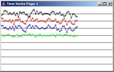 |
Figure 5
Error never goes to zero
One thing worth noting is that the error (green) never goes to zero in Figure 5 regardless of the quality of the adaptive solution. The target contains white random noise. There is nothing that the convolution filter being applied to chanA can do to eliminate that noise and it passes straight through from the target to the error in the subtraction process shown in Listing 26.
There is also white random noise on chanA. If the convolution filter maintains a flat amplitude response as intended, this noise will be passed through to the output also and will contribute to the noise on the error signal in Figure 5.
(Theoretically, however, the average of the white random noise from chanA and the white random noise from the target will be reduced by about the square root of 2 relative to the level on either channel.)
Despite the uncorrelated noise on both channels, the filtered output (red) is a reasonably good replica of the target (blue) by the beginning of the traces in the bottom page of Figure 5.
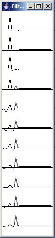
The impulse response
The impulse response at the beginning and at the end of every tenth adaptive iteration is shown in the left column in the two pages in Figure 6. As you can see, this impulse response is converted from a single impulse in the center of the convolution filter to a single impulse (plus a few very small non-zero values) three samples to the right of center after about 140 iterations. As you know, this is the correct solution, and it was achieved despite the presence of random noise on the two channels.
 |
 |
 |
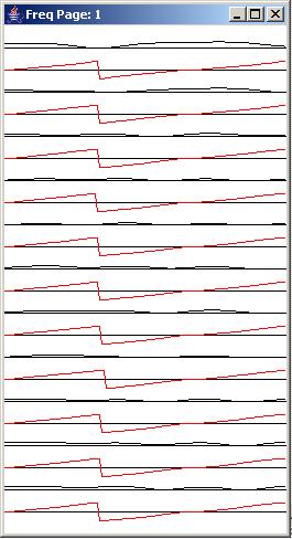 |
Figure 6
What this means is that after about 140 iterations, the output from the convolution filter has been shifted so as to register with the target. Most of the error that we see in Figure 5 after this point in time is simply the result of the random white noise being passed through from chanA and the target to the error.
The frequency response
After about 140 iterations, the amplitude response shown in the right column of Figure 6 is very flat, and the phase response has a positive slope and a linear shape indicating that the convolution filter has converged to the simple time-shift filter that we know to be the correct solution to the problem.
I encourage you to copy, compile and run the program provided in Listing 32 below. You will need some other classes in addition to the program in Listing 32.
I have provided the source code for the class named PlotALot05 in Listing 33. You will need to go to the previous lesson titled Plotting Large Quantities of Data using Java to get the source code for the other required PlotALot classes.
In addition, you will need to go to the lesson titled Spectrum Analysis using Java, Sampling Frequency, Folding Frequency, and the FFT Algorithm to get the source code for the class named ForwardRealToComplex01.
Have fun and learn
Above all, have fun and use this program to learn as much as you can about the basics of adaptive filtering.
In this lesson, I explained adaptive filtering using an LMS adaptive algorithm in a relatively simple scenario.
The next lesson will tackle a considerably more complicated scenario for adaptive filtering. In the next lesson, I will teach you how to write a whitening filter program for the extraction of wide band signals corrupted by narrow band noise.
Following that, the lessons in the series will become somewhat more general. I plan to publish lessons that explain and provide examples for the four common scenarios in which adaptive filtering is used:
Somewhere along the way I may publish a lesson that explains and illustrates the difference between least mean square (LMS) and recursive least squares (RLS) adaptive algorithms.
Complete listings of two of the programs discussed in this lesson are provided in Listing 32 and Listing 33 below.
/*File Adapt01.java.java
Copyright 2005, R.G.Baldwin
This program illustrates one aspect of time-
adaptive signal processing.
Two sampled time series, chanA and chanB,
are presented to the an adaptive algorithm. Each
time series contains the same wide band signal
plus white noise that is uncorrelated between the
two channels.
The signal in chanB may be delayed or advanced by
up to 6 samples relative to the signal in chanA.
A 9-point convolution operator is developed
adaptively. When the adaptive process converges
successflly, the time series produced by applying
the convolution operator to chanA matches the
signal on chanB.
The user provides the following information as
command line parameters:
timeShift - A negative value delays chanB
relative to chanA and a positive value advances
chanB relative to chanA. If no command line
parameters are provided, a default timeShift
value of -4 is used. This causes a four-sample
delay on chanB relative to chanA. Because the
convolution operator has only nine points, time
shifts greater than plus or minus four samples
cannot be resolved and an adaptive solution will
not be found. Time shifts greater than six
samples cause the program to terminate.
feedbackGain - Controls the convergence rate of
the adaptive process. If the value is very low,
the process will take a long time to converge.
If the value is too high, the process will become
unstable. If no command line parameters are
provided, a feedbackGain value of 0.001 is used.
Depending on the random noise level, the process
appears to be stable for feedbackGain values as
large as 0.004, but goes unstable for a
feedbackGain value of 0.005.
noiseLevel - Controls the amount of uncorrelated
white noise that is added to the signal on each
of the channels. If no command line parameters
are provided, the default noise level is 0.0 The
noise level is provided as a decimal fraction of
the signal level. For example, a noise level
of 0.1 causes the level of the noise that is
added to each of the channels to be one tenth of
the signal level on that channel.
numberIterations - The number of adaptive
iterations performed before the adaptive process
terminates and all of the data that has been
saved is plotted. If no command line parameters
are provided, the default is 100 iterations.
The following time series are plotted in color
showing the convergence of the adaptive
algorithm:
black: input to the filter
red: output from the filter
blue: adaptive target
green: error
In addition, the frequency response of the filter
at the beginning and at the end of every tenth
iteration is computed and displayed when the
adaptive process terminates. Both the amplitude
and the phase response of the filter are computed
and plotted. Also, the filter is plotted as a
time series on the same iterations that the
frequency response is computed. Thus, the shape
of the filter can be compared with the frequency
response of the filter.
The filter is initialized with a single
coefficient value of 1 at the center and 0 for
all of the other coefficient values. The ideal
solution is a single coefficient value of 1 at a
location in the filter that matches the time
shift between chanA and the target. The value
of 1 can be seen to progress from the center of
the filter to the correct location in the filter
as the program iterates. In addition, the phase
response can be seen to change appropriately as
the program iterates.
Tested using J2SE 5.0 and WinXP
J2SE 5.0 or later is required.
************************************************/
import static java.lang.Math.*;//J2SE 5.0 req
class Adapt01{
public static void main(String[] args){
//Default values
int timeShift = -4;
double feedbackGain = 0.001;
double noiseLevel = 0.0;
int numberIterations = 100;
if(args.length != 4){
System.out.println(
"Usage: java Adapt01 " +
"timeShift feedbackGain " +
"noiseLevel numberIterations");
System.out.println(
"Negative timeShift is delay");
System.out.println(
"Using -4 sample shift by default");
System.out.println(
"Using 0.001 feedbackGain by default");
System.out.println(
"noiseLevel is a decimal fraction");
System.out.println("Using 0.0 by default");
System.out.println(
"numberIterations is an int");
System.out.println("Using 100 by default");
}else{//Command line params were provided.
//Convert String to int
timeShift = Integer.parseInt(args[0]);
System.out.println(
"timeShift: " + timeShift);
//Convert String to double
feedbackGain = Double.parseDouble(args[1]);
System.out.println(
"feedbackGain: " + feedbackGain);
//Convert String to double
noiseLevel = Double.parseDouble(args[2]);
System.out.println(
"noiseLevel: " + noiseLevel);
//Convert String to int
numberIterations =
Integer.parseInt(args[3]);
System.out.println(
"numberIterations: " + numberIterations);
}//end else
if(abs(timeShift) > 6){
System.out.println(
"Time shift magnitude > 6 not allowed.");
System.out.println("Terminating");
System.exit(0);
}//end if
//Instantiate an object of the class and
// execute the adaptive algorithm using the
// specified feedbackGain and other
// parameters.
new Adapt01().process(timeShift,
feedbackGain,
noiseLevel,
numberIterations);
}//end main
//-------------------------------------------//
void process(int timeShift,
double feedbackGain,
double noiseLevel,
int numberIterations){
//The process begins with a filter having
// the following initial coefficients.
double[] filter = {0,0,0,0,1,0,0,0,0};
//Create array objects that will be used as
// delay lines.
double[] rawData = new double[13];
double[] chanA = new double[9];
double[] chanB = new double[9];
//Instantiate a plotting object for four
// data channels. This object will be used
// to plot the time series data.
PlotALot05 plotObj = new PlotALot05(
"Time Series",398,250,25,5,4,4);
//Instantiate a plotting object for two
// channels of filter frequency response
// data. One channel is used to plot the
// amplitude response in db and the other
// channel is used to plot the phase on a
// scale that extends from -180 degrees to
// +180 degrees.
PlotALot03 freqPlotObj =
new PlotALot03("Freq",264,487,20,2,0,0);
//Instantiate a plotting object to display
// the filter as a short time series at
// intervals during the adaptive process.
// Note that the minimum allowable width
// for a Frame is 112 pixels under WinXP.
// Therefore, the following display doesn't
// synchronize properly for filter lengths
// less than 25 coefficients. However, the
// code that feeds the filter data to the
// plotting object later in the program
// extends the length of the filter to
// cause it to synchronize and to plot one
// set of filter coefficients on each axis.
PlotALot01 filterPlotObj = new PlotALot01(
"Filter",(filter.length * 4) + 8,
487,40,4,0,0);
//Display frequency response of initial
// filter computed at 128 points between zero
// and the folding frequency.
displayFreqResponse(filter,
freqPlotObj,
128,
filter.length - 5);
//Display the initial filter as a time series
// on the first axis.
for(int cnt = 0;cnt < filter.length;cnt++){
filterPlotObj.feedData(30*filter[cnt]);
}//end for loop
//Extend the filter with a value of 2.5 for
// plotting to cause it to synchronize
// properly with the plotting software. See
// earlier comment on this topic. Note that
// this will not cause the plot to
// synchronize properly on an operating
// system for which the sum of the left and
// right insets on a Frame object are
// different from 8 pixels.
if(filter.length <= 26){
for(int cnt = 0;cnt < (26 - filter.length);
cnt++){
filterPlotObj.feedData(2.5);
}//end for loop
}//end if
//Declare and initialize variables used in
// the adaptive process.
double output = 0;
double err = 0;
double target = 0;
double input = 0;
double dataScale = 25;//Default data scale
//Do the iterative adaptive process
for(int cnt = 0;cnt < numberIterations;
cnt++){
//Add new input data to the delay line
// containing the raw input data.
flowLine(rawData,Math.random() - 0.5);
//Extract the middle sample from the input
// data delay line, add some random noise,
// and insert it into the delay line
// containing the data for chanA.
flowLine(chanA,dataScale*rawData[6] +
noiseLevel*dataScale*(Math.random()
- 0.5));
//Extract data with a time shift from the
// input data delay line, add some random
// noise, and insert it into the delay line
// containing the data for chanB.
flowLine(chanB,
dataScale*rawData[6 + timeShift] +
noiseLevel*dataScale*(Math.random()
- 0.5));
//Get the middle sample from the chanA
// delay line for plotting.
input = chanA[chanA.length/2];
//Apply the current filter coefficients to
// the chanA data contained in the delay
// line.
output = dotProduct(filter,chanA);
//Get the middle sample from the chanB
// delay line and use it as the adaptive
// target. In other words, the adaptive
// process will attempt to cause the
// filtered output to match the value in
// the middle of the chanB delay line.
target = chanB[chanB.length/2];
//Compute the error between the current
// filter output and the target.
err = output - target;
//Update the filter coefficients
for(int ctr = 0;ctr < filter.length;ctr++){
filter[ctr] -=
err*chanA[ctr]*feedbackGain;
}//end for loop
//This is the end of the adaptive process.
// The code beyond this point is used to
// display information about the adaptive
// process.
//Feed the time series data to the plotting
// object.
plotObj.feedData(input,output,target,err);
//Compute and plot the frequency response
// and plot the filter as a time series
// every 10 iterations.
if(cnt%10 == 0){
displayFreqResponse(filter,
freqPlotObj,
128,
filter.length - 5);
//Plot the filter coefficient values.
// Scale the coefficient values by 30
// to make them compatible with the
// plotting software.
for(int ctr = 0;ctr < filter.length;
ctr++){
filterPlotObj.feedData(30*filter[ctr]);
}//end for loop
//Extend the filter with a value of 2.5
// for plotting to cause it to
// synchronize with one filter on each
// axis. See explanatory comment
// earlier.
if(filter.length <= 26){
for(int count = 0;
count < (26 - filter.length);
count++){
filterPlotObj.feedData(2.5);
}//end for loop
}//end if
}//end if on cnt%10
}//end for loop
//Cause all the data to be plotted in the
// screen locations specified.
plotObj.plotData();
freqPlotObj.plotData(0,201);
filterPlotObj.plotData(265,201);
}//end process
//-------------------------------------------//
//This method simulates a tapped delay line.
// It receives a reference to an array and
// a value. It discards the value at
// index 0 of the array, moves all the other
// values by one element toward 0, and
// inserts the new value at the top of the
// array.
void flowLine(double[] line,double val){
for(int cnt = 0;cnt < (line.length - 1);
cnt++){
line[cnt] = line[cnt+1];
}//end for loop
line[line.length - 1] = val;
}//end flowLine
//-------------------------------------------//
//This method receives two arrays and treats
// the first n elements in each array as a pair
// of vectors. It computes and returns the
// vector dot product of the two vectors. If
// the length of one array is greater than the
// length of the other array, it considers the
// number of dimensions of the vectors to be
// equal to the length of the smaller array.
double dotProduct(double[] v1,double[] v2){
double result = 0;
if((v1.length) <= (v2.length)){
for(int cnt = 0;cnt < v1.length;cnt++){
result += v1[cnt]*v2[cnt];
}//end for loop
return result;
}else{
for(int cnt = 0;cnt < v2.length;cnt++){
result += v1[cnt]*v2[cnt];
}//end for loop
return result;
}//end else
}//end dotProduct
//-------------------------------------------//
//This method receives a reference to a double
// array containing a convolution filter
// along with a reference to a plotting object
// capable of plotting two channels of data.
// It also receives a value specifying the
// number of frequencies at which a DFT is
// to be performed on the filter, along with
// the sample number that represents the zero
// time location in the filter. The method
// uses this information to perform a DFT on
// the filter from zero to the folding
// frequency. It feeds the amplitude spectrum
// and the phase spectrum to the plotting
// object for plotting.
void displayFreqResponse(double[] filter,
PlotALot03 plot,
int len,
int zeroTime){
//Create the arrays required by the Fourier
// Transform.
double[] timeDataIn = new double[len];
double[] realSpect = new double[len];
double[] imagSpect = new double[len];
double[] angle = new double[len];
double[] magnitude = new double[len];
//Copy the filter into the timeDataIn array.
System.arraycopy(filter,0,timeDataIn,0,
filter.length);
//Compute DFT of the filter from zero to the
// folding frequency and save it in the
// output arrays.
ForwardRealToComplex01.transform(timeDataIn,
realSpect,
imagSpect,
angle,
magnitude,
zeroTime,
0.0,
0.5);
//Plot the magnitude data. Convert to
// normalized decibels before plotting.
//Eliminate or change all values that are
// incompatible with log10 method.
for(int cnt = 0;cnt < magnitude.length;
cnt++){
if((magnitude[cnt] == Double.NaN) ||
(magnitude[cnt] <= 0)){
magnitude[cnt] = 0.0000001;
}else if(magnitude[cnt] ==
Double.POSITIVE_INFINITY){
magnitude[cnt] = 9999999999.0;
}//end else if
}//end for loop
//Now convert magnitude data to log base 10
for(int cnt = 0;cnt < magnitude.length;
cnt++){
magnitude[cnt] = log10(magnitude[cnt]);
}//end for loop
//Note that from this point forward, all
// references to magnitude are referring to
// log base 10 data, which can be thought of
// as scaled decibels.
//Find the absolute peak value
double peak = -9999999999.0;
for(int cnt = 0;cnt < magnitude.length;
cnt++){
if(peak < abs(magnitude[cnt])){
peak = abs(magnitude[cnt]);
}//end if
}//end for loop
//Normalize to 50 times the peak value and
// shift up the screen by 50 units to make
// the values compatible with the plotting
// program. Recall that adding a constant to
// log values is equivalent to scaling the
// original data.
for(int cnt = 0;cnt < magnitude.length;
cnt++){
magnitude[cnt] =
50*magnitude[cnt]/peak + 50;
}//end for loop
//Now feed the normalized decibel data to the
// plotting object. The angle data ranges
// from -180 to +180. Scale it down by a
// factor of 20 to make it compatible with
// the plotting format being used.
for(int cnt = 0;cnt < magnitude.length;
cnt++){
plot.feedData(
magnitude[cnt],angle[cnt]/20);
}//end for loop
}//end displayFreqResponse
//-------------------------------------------//
}//end class Adapt01 |
/*File PlotALot05.java
Copyright 2005, R.G.Baldwin
This program is an update to the program named
PlotALot04 for the purpose of plotting four
data channels. See PlotALot04 for descriptive
comments. Otherwise, the comments in this
program have not been updated to reflect this
update.
The program was tested using J2SE 5.0 and WinXP.
Requires J2SE 5.0 to support generics.
************************************************/
import java.awt.*;
import java.awt.event.*;
import java.util.*;
public class PlotALot05{
//This main method is provided so that the
// class can be run as an application to test
// itself.
public static void main(String[] args){
//Instantiate a plotting object using the
// version of the constructor that allows for
// controlling the plotting parameters.
PlotALot05 plotObjectA =
new PlotALot05("A",158,250,25,5,4,4);
//Feed quadruplets of data values to the
// plotting object.
for(int cnt = 0;cnt < 115;cnt++){
//Plot some white random noise. Note that
// fifteen of the values for each time
// series are not random. See the opening
// comments for a discussion of the reasons
// why.
double valBlack = (Math.random() - 0.5)*25;
double valRed = valBlack;
double valBlue = valBlack;
double valGreen = valBlack;
//Feed quadruplets of values to the
// plotting object by invoking the feedData
// method once for each quadruplet of data
// values.
if(cnt == 57){
plotObjectA.feedData(0,0,0,0);
}else if(cnt == 58){
plotObjectA.feedData(0,0,0,0);
}else if(cnt == 59){
plotObjectA.feedData(25,25,25,25);
}else if(cnt == 60){
plotObjectA.feedData(-25,-25,-25,-25);
}else if(cnt == 61){
plotObjectA.feedData(25,25,25,25);
}else if(cnt == 62){
plotObjectA.feedData(0,0,0,0);
}else if(cnt == 63){
plotObjectA.feedData(0,0,0,0);
}else if(cnt == 26){
plotObjectA.feedData(0,0,0,0);
}else if(cnt == 27){
plotObjectA.feedData(0,0,0,0);
}else if(cnt == 28){
plotObjectA.feedData(20,20,20,20);
}else if(cnt == 29){
plotObjectA.feedData(20,20,20,20);
}else if(cnt == 30){
plotObjectA.feedData(-20,-20,-20,-20);
}else if(cnt == 31){
plotObjectA.feedData(-20,-20,-20,-20);
}else if(cnt == 32){
plotObjectA.feedData(0,0,0,0);
}else if(cnt == 33){
plotObjectA.feedData(0,0,0,0);
}else{
plotObjectA.feedData(valBlack,
valRed,
valBlue,
valGreen);
}//end else
}//end for loop
//Cause the data to be plotted in the default
// screen location.
plotObjectA.plotData();
}//end main
//-------------------------------------------//
String title;
int frameWidth;
int frameHeight;
int traceSpacing;//pixels between traces
int sampSpacing;//pixels between samples
int ovalWidth;//width of sample marking oval
int ovalHeight;//height of sample marking oval
int tracesPerPage;
int samplesPerPage;
int pageCounter = 0;
int sampleCounter = 0;
ArrayList <Page> pageLinks =
new ArrayList<Page>();
//There are two overloaded versions of the
// constructor for this class. This
// overloaded version accepts several incoming
// parameters allowing the user to control
// various aspects of the plotting format. A
// different overloaded version accepts a title
// string only and sets all of the plotting
// parameters to default values.
PlotALot05(String title,//Frame title
int frameWidth,//in pixels
int frameHeight,//in pixels
int traceSpacing,//in pixels
int sampSpace,//in pixels per sample
int ovalWidth,//sample marker width
int ovalHeight)//sample marker hite
{//constructor
//Specify sampSpace as pixels per sample.
// Should never be less than 1. Convert to
// pixels between samples for purposes of
// computation.
this.title = title;
this.frameWidth = frameWidth;
this.frameHeight = frameHeight;
this.traceSpacing = traceSpacing;
//Convert to pixels between samples.
this.sampSpacing = sampSpace - 1;
this.ovalWidth = ovalWidth;
this.ovalHeight = ovalHeight;
//The following object is instantiated solely
// to provide information about the width and
// height of the canvas. This information is
// used to compute a variety of other
// important values.
Page tempPage = new Page(title);
int canvasWidth = tempPage.canvas.getWidth();
int canvasHeight =
tempPage.canvas.getHeight();
//Display information about this plotting
// object.
System.out.println("\nTitle: " + title);
System.out.println(
"Frame width: " + tempPage.getWidth());
System.out.println(
"Frame height: " + tempPage.getHeight());
System.out.println(
"Page width: " + canvasWidth);
System.out.println(
"Page height: " + canvasHeight);
System.out.println(
"Trace spacing: " + traceSpacing);
System.out.println(
"Sample spacing: " + (sampSpacing + 1));
if(sampSpacing < 0){
System.out.println("Terminating");
System.exit(0);
}//end if
//Get rid of this temporary page.
tempPage.dispose();
//Now compute the remaining important values.
tracesPerPage =
(canvasHeight - traceSpacing/2)/
traceSpacing;
System.out.println("Traces per page: "
+ tracesPerPage);
if((tracesPerPage == 0) ||
(tracesPerPage%4 != 0) ){
System.out.println("Terminating program");
System.exit(0);
}//end if
samplesPerPage = canvasWidth * tracesPerPage/
(sampSpacing + 1)/4;
System.out.println("Samples per page: "
+ samplesPerPage);
//Now instantiate the first usable Page
// object and store its reference in the
// list.
pageLinks.add(new Page(title));
}//end constructor
//-------------------------------------------//
PlotALot05(String title){
//Invoke the other overloaded constructor
// passing default values for all but the
// title.
this(title,400,410,50,2,2,2);
}//end overloaded constructor
//-------------------------------------------//
//Invoke this method once for each quadruplet
// of data values to be plotted.
void feedData(double valBlack,
double valRed,
double valBlue,
double valGreen){
if((sampleCounter) == samplesPerPage){
//if the page is full, increment the page
// counter, create a new empty page, and
// reset the sample counter.
pageCounter++;
sampleCounter = 0;
pageLinks.add(new Page(title));
}//end if
//Store the sample values in the MyCanvas
// object to be used later to paint the
// screen. Then increment the sample
// counter. The sample values pass through
// the page object into the current MyCanvas
// object.
pageLinks.get(pageCounter).putData(
valBlack,
valRed,
valBlue,
valGreen,
sampleCounter);
sampleCounter++;
}//end feedData
//-------------------------------------------//
//There are two overloaded versions of the
// plotData method. One version allows the
// user to specify the location on the screen
// where the stack of plotted pages will
// appear. The other version places the stack
// in the upper left corner of the screen.
//Invoke one of the overloaded versions of
// this method once when all data has been fed
// to the plotting object in order to rearrange
// the order of the pages with page 0 at the
// top of the stack on the screen.
//For this overloaded version, specify xCoor
// and yCoor to control the location of the
// stack on the screen. Values of 0,0 will
// place the stack at the upper left corner of
// the screen. Also see the other overloaded
// version, which places the stack at the upper
// left corner of the screen by default.
void plotData(int xCoor,int yCoor){
Page lastPage =
pageLinks.get(pageLinks.size() - 1);
//Delay until last page becomes visible.
while(!lastPage.isVisible()){
//Loop until last page becomes visible
}//end while loop
Page tempPage = null;
//Make all pages invisible
for(int cnt = 0;cnt < (pageLinks.size());
cnt++){
tempPage = pageLinks.get(cnt);
tempPage.setVisible(false);
}//end for loop
//Now make all pages visible in reverse order
// so that page 0 will be on top of the
// stack on the screen.
for(int cnt = pageLinks.size() - 1;cnt >= 0;
cnt--){
tempPage = pageLinks.get(cnt);
tempPage.setLocation(xCoor,yCoor);
tempPage.setVisible(true);
}//end for loop
}//end plotData(int xCoor,int yCoor)
//-------------------------------------------//
//This overloaded version of the method causes
// the stack to be located in the upper left
// corner of the screen by default
void plotData(){
plotData(0,0);//invoke overloaded version
}//end plotData()
//-------------------------------------------//
//Inner class. A PlotALot05 object may
// have as many Page objects as are required
// to plot all of the data values. The
// reference to each Page object is stored
// in an ArrayList object belonging to the
// PlotALot05 object.
class Page extends Frame{
MyCanvas canvas;
int sampleCounter;
Page(String title){//constructor
canvas = new MyCanvas();
add(canvas);
setSize(frameWidth,frameHeight);
setTitle(title + " Page: " + pageCounter);
setVisible(true);
//---------------------------------------//
//Anonymous inner class to terminate the
// program when the user clicks the close
// button on the Frame.
addWindowListener(
new WindowAdapter(){
public void windowClosing(
WindowEvent e){
System.exit(0);//terminate program
}//end windowClosing()
}//end WindowAdapter
);//end addWindowListener
//---------------------------------------//
}//end constructor
//=========================================//
//This method receives a quadruplet of sample
// values of type double and stores each of
// them in a separate array object belonging
// to the MyCanvas object.
void putData(double valBlack,
double valRed,
double valBlue,
double valGreen,
int sampleCounter){
canvas.blackData[sampleCounter] = valBlack;
canvas.redData[sampleCounter] = valRed;
canvas.blueData[sampleCounter] = valBlue;
canvas.greenData[sampleCounter] = valGreen;
//Save the sample counter in an instance
// variable to make it available to the
// overridden paint method. This value is
// needed by the paint method so it will
// know how many samples to plot on the
// final page which probably won't be full.
this.sampleCounter = sampleCounter;
}//end putData
//=========================================//
//Inner class
class MyCanvas extends Canvas{
double [] blackData =
new double[samplesPerPage];
double [] redData =
new double[samplesPerPage];
double [] blueData =
new double[samplesPerPage];
double [] greenData =
new double[samplesPerPage];
//Override the paint method
public void paint(Graphics g){
//Draw horizontal axes, one for each
// trace.
for(int cnt = 0;cnt < tracesPerPage;
cnt++){
g.drawLine(0,
(cnt+1)*traceSpacing,
this.getWidth(),
(cnt+1)*traceSpacing);
}//end for loop
//Plot the points if there are any to be
// plotted.
if(sampleCounter > 0){
for(int cnt = 0;cnt <= sampleCounter;
cnt++){
//Begin by plotting the values from
// the blackData array object.
g.setColor(Color.BLACK);
//Compute a vertical offset to locate
// the black data on every third axis
// on the page.
int yOffset =
((1 + cnt*(sampSpacing + 1)/
this.getWidth())*4*traceSpacing)
- 3*traceSpacing;
//Draw an oval centered on the sample
// value to mark the sample in the
// plot. It is best if the dimensions
// of the oval are evenly divisable
// by 2 for centering purposes.
//Reverse the sign of the sample
// value to cause positive sample
// values to be plotted above the
// axis.
g.drawOval(cnt*(sampSpacing + 1)%
this.getWidth() - ovalWidth/2,
yOffset - (int)blackData[cnt]
- ovalHeight/2,
ovalWidth,
ovalHeight);
//Connect the sample values with
// straight lines. Do not draw a
// line connecting the last sample in
// one trace to the first sample in
// the next trace.
if(cnt*(sampSpacing + 1)%
this.getWidth() >=
sampSpacing + 1){
g.drawLine(
(cnt - 1)*(sampSpacing + 1)%
this.getWidth(),
yOffset - (int)blackData[cnt-1],
cnt*(sampSpacing + 1)%
this.getWidth(),
yOffset - (int)blackData[cnt]);
}//end if
//Now plot the data stored in the
// redData array object.
g.setColor(Color.RED);
//Compute a vertical offset to locate
// the red data on every third axis
// on the page.
yOffset = (1 + cnt*(sampSpacing + 1)/
this.getWidth())*4*traceSpacing
- 2*traceSpacing;
//Draw the ovals as described above.
g.drawOval(cnt*(sampSpacing + 1)%
this.getWidth() - ovalWidth/2,
yOffset - (int)redData[cnt]
- ovalHeight/2,
ovalWidth,
ovalHeight);
//Connect the sample values with
// straight lines as described above.
if(cnt*(sampSpacing + 1)%
this.getWidth() >=
sampSpacing + 1){
g.drawLine(
(cnt - 1)*(sampSpacing + 1)%
this.getWidth(),
yOffset - (int)redData[cnt-1],
cnt*(sampSpacing + 1)%
this.getWidth(),
yOffset - (int)redData[cnt]);
}//end if
//Now plot the data stored in the
// blueData array object.
g.setColor(Color.BLUE);
//Compute a vertical offset to locate
// the blue data on every third axis
// on the page.
yOffset = (1 + cnt*(sampSpacing + 1)/
this.getWidth())*4*traceSpacing
-traceSpacing;
//Draw the ovals as described above.
g.drawOval(cnt*(sampSpacing + 1)%
this.getWidth() - ovalWidth/2,
yOffset - (int)blueData[cnt]
- ovalHeight/2,
ovalWidth,
ovalHeight);
//Connect the sample values with
// straight lines as described above.
if(cnt*(sampSpacing + 1)%
this.getWidth() >=
sampSpacing + 1){
g.drawLine(
(cnt - 1)*(sampSpacing + 1)%
this.getWidth(),
yOffset - (int)blueData[cnt-1],
cnt*(sampSpacing + 1)%
this.getWidth(),
yOffset - (int)blueData[cnt]);
}//end if
//Now plot the data stored in the
// greenData array object.
g.setColor(Color.GREEN);
//Compute a vertical offset to locate
// the green data on every third axis
// on the page.
yOffset = (1 + cnt*(sampSpacing + 1)/
this.getWidth())*4*traceSpacing;
//Draw the ovals as described above.
g.drawOval(cnt*(sampSpacing + 1)%
this.getWidth() - ovalWidth/2,
yOffset - (int)greenData[cnt]
- ovalHeight/2,
ovalWidth,
ovalHeight);
//Connect the sample values with
// straight lines as described above.
if(cnt*(sampSpacing + 1)%
this.getWidth() >=
sampSpacing + 1){
g.drawLine(
(cnt - 1)*(sampSpacing + 1)%
this.getWidth(),
yOffset - (int)greenData[cnt-1],
cnt*(sampSpacing + 1)%
this.getWidth(),
yOffset - (int)greenData[cnt]);
}//end if
}//end for loop
}//end if for sampleCounter > 0
}//end overridden paint method
}//end inner class MyCanvas
}//end inner class Page
}//end class PlotALot05
//=============================================// |
Copyright 2005, Richard G. Baldwin. Reproduction in whole or in part in any form or medium without express written permission from Richard Baldwin is prohibited.
Richard has participated in numerous consulting projects and he frequently provides onsite training at the high-tech companies located in and around Austin, Texas. He is the author of Baldwin's Programming Tutorials, which has gained a worldwide following among experienced and aspiring programmers. He has also published articles in JavaPro magazine.
In addition to his programming expertise, Richard has many years of practical experience in Digital Signal Processing (DSP). His first job after he earned his Bachelor's degree was doing DSP in the Seismic Research Department of Texas Instruments. (TI is still a world leader in DSP.) In the following years, he applied his programming and DSP expertise to other interesting areas including sonar and underwater acoustics.
Richard holds an MSEE degree from Southern Methodist University and has many years of experience in the application of computer technology to real-world problems.
Keywords
Java adaptive filtering convolution filter frequency spectrum LMS amplitude
phase time-delay linear DSP impulse decibel log10 DFT transform bandwidth signal
noise real-time dot-product vector time-series
-end-