

| << Chapter < Page | Chapter >> Page > |
| Wage | Quantity Labor Demanded | Quantity Labor Supplied |
|---|---|---|
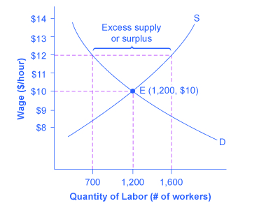
| $8/hr | 1,900 | 500 |
| $9/hr | 1,500 | 900 |
| $10/hr | 1,200 | 1,200 |
| $11/hr | 900 | 1,400 |
| $12/hr | 700 | 1,600 |
| $13/hr | 500 | 1,800 |
| $14/hr | 400 | 1,900 |
The U.S. minimum wage is a price floor that is set either very close to the equilibrium wage or even slightly below it. About 1% of American workers are actually paid the minimum wage. In other words, the vast majority of the U.S. labor force has its wages determined in the labor market, not as a result of the government price floor. But for workers with low skills and little experience, like those without a high school diploma or teenagers, the minimum wage is quite important. In many cities, the federal minimum wage is apparently below the market price for unskilled labor, because employers offer more than the minimum wage to checkout clerks and other low-skill workers without any government prodding.
Economists have attempted to estimate how much the minimum wage reduces the quantity demanded of low-skill labor. A typical result of such studies is that a 10% increase in the minimum wage would decrease the hiring of unskilled workers by 1 to 2%, which seems a relatively small reduction. In fact, some studies have even found no effect of a higher minimum wage on employment at certain times and places—although these studies are controversial.
Let’s suppose that the minimum wage lies just slightly below the equilibrium wage level. Wages could fluctuate according to market forces above this price floor, but they would not be allowed to move beneath the floor. In this situation, the price floor minimum wage is said to be nonbinding —that is, the price floor is not determining the market outcome. Even if the minimum wage moves just a little higher, it will still have no effect on the quantity of employment in the economy, as long as it remains below the equilibrium wage. Even if the minimum wage is increased by enough so that it rises slightly above the equilibrium wage and becomes binding, there will be only a small excess supply gap between the quantity demanded and quantity supplied.
These insights help to explain why U.S. minimum wage laws have historically had only a small impact on employment. Since the minimum wage has typically been set close to the equilibrium wage for low-skill labor and sometimes even below it, it has not had a large effect in creating an excess supply of labor. However, if the minimum wage were increased dramatically—say, if it were doubled to match the living wages that some U.S. cities have considered—then its impact on reducing the quantity demanded of employment would be far greater. The following Clear It Up feature describes in greater detail some of the arguments for and against changes to minimum wage.
Because of the law of demand, a higher required wage will reduce the amount of low-skill employment either in terms of employees or in terms of work hours. Although there is controversy over the numbers, let’s say for the sake of the argument that a 10% rise in the minimum wage will reduce the employment of low-skill workers by 2%. Does this outcome mean that raising the minimum wage by 10% is bad public policy? Not necessarily.
If 98% of those receiving the minimum wage have a pay increase of 10%, but 2% of those receiving the minimum wage lose their jobs, are the gains for society as a whole greater than the losses? The answer is not clear, because job losses, even for a small group, may cause more pain than modest income gains for others. For one thing, we need to consider which minimum wage workers are losing their jobs. If the 2% of minimum wage workers who lose their jobs are struggling to support families, that is one thing. If those who lose their job are high school students picking up spending money over summer vacation, that is something else.
Another complexity is that many minimum wage workers do not work full-time for an entire year. Imagine a minimum wage worker who holds different part-time jobs for a few months at a time, with bouts of unemployment in between. The worker in this situation receives the 10% raise in the minimum wage when working, but also ends up working 2% fewer hours during the year because the higher minimum wage reduces how much employers want people to work. Overall, this worker’s income would rise because the 10% pay raise would more than offset the 2% fewer hours worked.
Of course, these arguments do not prove that raising the minimum wage is necessarily a good idea either. There may well be other, better public policy options for helping low-wage workers. (The Poverty and Economic Inequality chapter discusses some possibilities.) The lesson from this maze of minimum wage arguments is that complex social problems rarely have simple answers. Even those who agree on how a proposed economic policy affects quantity demanded and quantity supplied may still disagree on whether the policy is a good idea.
In the labor market, households are on the supply side of the market and firms are on the demand side. In the market for financial capital, households and firms can be on either side of the market: they are suppliers of financial capital when they save or make financial investments, and demanders of financial capital when they borrow or receive financial investments.
In the demand and supply analysis of labor markets, the price can be measured by the annual salary or hourly wage received. The quantity of labor can be measured in various ways, like number of workers or the number of hours worked.
Factors that can shift the demand curve for labor include: a change in the quantity demanded of the product that the labor produces; a change in the production process that uses more or less labor; and a change in government policy that affects the quantity of labor that firms wish to hire at a given wage. Demand can also increase or decrease (shift) in response to: workers’ level of education and training, technology, the number of companies, and availability and price of other inputs.
The main factors that can shift the supply curve for labor are: how desirable a job appears to workers relative to the alternatives, government policy that either restricts or encourages the quantity of workers trained for the job, the number of workers in the economy, and required education.
Identify each of the following as involving either demand or supply. Draw a circular flow diagram and label the flows A through F. (Some choices can be on both sides of the goods market.)
Predict how each of the following events will raise or lower the equilibrium wage and quantity of coal miners in West Virginia. In each case, sketch a demand and supply diagram to illustrate your answer.
American Community Survey. 2012. "School Enrollment and Work Status: 2011." Accessed April 13, 2015. http://www.census.gov/prod/2013pubs/acsbr11-14.pdf.
National Center for Educational Statistics. “Digest of Education Statistics.” (2008 and 2010). Accessed December 11, 2013. nces.ed.gov.
Notification Switch
Would you like to follow the 'Microeconomics' conversation and receive update notifications?

|
|

|
|

|
|

|
|

|
|

|
|

|
|

|
|

|
|

|
|

|