

| << Chapter < Page | Chapter >> Page > |
Tax policy can affect consumption and investment spending, too. Tax cuts for individuals will tend to increase consumption demand, while tax increases will tend to diminish it. Tax policy can also pump up investment demand by offering lower tax rates for corporations or tax reductions that benefit specific kinds of investment. Shifting C or I will shift the AD curve as a whole.
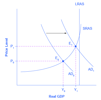
During a recession , when unemployment is high and many businesses are suffering low profits or even losses, the U.S. Congress often passes tax cuts. During the recession of 2001, for example, a tax cut was enacted into law. At such times, the political rhetoric often focuses on how people going through hard times need relief from taxes. The aggregate supply and aggregate demand framework, however, offers a complementary rationale, as illustrated in [link] . The original equilibrium during a recession is at point E 0 , relatively far from the full employment level of output. The tax cut, by increasing consumption, shifts the AD curve to the right. At the new equilibrium (E 1 ), real GDP rises and unemployment falls and, because in this diagram the economy has not yet reached its potential or full employment level of GDP, any rise in the price level remains muted. Read the following Clear It Up feature to consider the question of whether economists favor tax cuts or oppose them.
One of the most fundamental divisions in American politics over the last few decades has been between those who believe that the government should cut taxes substantially and those who disagree. Ronald Reagan rode into the presidency in 1980 partly because of his promise, soon carried out, to enact a substantial tax cut. George Bush lost his bid for reelection against Bill Clinton in 1992 partly because he had broken his 1988 promise: “Read my lips! No new taxes!” In the 2000 presidential election, both George W. Bush and Al Gore advocated substantial tax cuts and Bush succeeded in pushing a package of tax cuts through Congress early in 2001. Disputes over tax cuts often ignite at the state and local level as well.
What side are economists on? Do they support broad tax cuts or oppose them? The answer, unsatisfying to zealots on both sides, is that it depends. One issue is whether the tax cuts are accompanied by equally large government spending cuts. Economists differ, as does any broad cross-section of the public, on how large government spending should be and what programs might be cut back. A second issue, more relevant to the discussion in this chapter, concerns how close the economy is to the full employment level of output. In a recession, when the intersection of the AD and AS curves is far below the full employment level, tax cuts can make sense as a way of shifting AD to the right. However, when the economy is already doing extremely well, tax cuts may shift AD so far to the right as to generate inflationary pressures, with little gain to GDP.
With the AD/AS framework in mind, many economists might readily believe that the Reagan tax cuts of 1981, which took effect just after two serious recessions, were beneficial economic policy. Similarly, the Bush tax cuts of 2001 and the Obama tax cuts of 2009 were enacted during recessions. However, some of the same economists who favor tax cuts in time of recession would be much more dubious about identical tax cuts at a time the economy is performing well and cyclical unemployment is low.
The use of government spending and tax cuts can be a useful tool to affect aggregate demand and it will be discussed in greater detail in the Government Budgets and Fiscal Policy chapter and The Impacts of Government Borrowing . Other policy tools can shift the aggregate demand curve as well. For example, as discussed in the Monetary Policy and Bank Regulation chapter, the Federal Reserve can affect interest rates and the availability of credit. Higher interest rates tend to discourage borrowing and thus reduce both household spending on big-ticket items like houses and cars and investment spending by business. Conversely, lower interest rates will stimulate consumption and investment demand. Interest rates can also affect exchange rates, which in turn will have effects on the export and import components of aggregate demand.
Spelling out the details of these alternative policies and how they affect the components of aggregate demand can wait for The Keynesian Perspective chapter. Here, the key lesson is that a shift of the aggregate demand curve to the right leads to a greater real GDP and to upward pressure on the price level. Conversely, a shift of aggregate demand to the left leads to a lower real GDP and a lower price level. Whether these changes in output and price level are relatively large or relatively small, and how the change in equilibrium relates to potential GDP, depends on whether the shift in the AD curve is happening in the relatively flat or relatively steep portion of the AS curve.
The AD curve will shift out as the components of aggregate demand—C, I, G, and X–M—rise. It will shift back to the left as these components fall. These factors can change because of different personal choices, like those resulting from consumer or business confidence, or from policy choices like changes in government spending and taxes. If the AD curve shifts to the right, then the equilibrium quantity of output and the price level will rise. If the AD curve shifts to the left, then the equilibrium quantity of output and the price level will fall. Whether equilibrium output changes relatively more than the price level or whether the price level changes relatively more than output is determined by where the AD curve intersects with the AS curve.
The AD/AS diagram superficially resembles the microeconomic supply and demand diagram on the surface, but in reality, what is on the horizontal and vertical axes and the underlying economic reasons for the shapes of the curves are very different. Long-term economic growth is illustrated in the AD/AS framework by a gradual shift of the aggregate supply curve to the right. A recession is illustrated when the intersection of AD and AS is substantially below potential GDP, while an expanding economy is illustrated when the intersection of AS and AD is near potential GDP.
Notification Switch
Would you like to follow the 'Macroeconomics' conversation and receive update notifications?

|
|
|
|
|

|
|

|
|

|
|

|
|

|
|

|
|

|
|

|
|

|
|

|