

| << Chapter < Page | Chapter >> Page > |
Taking both effects together, the substitution effect is encouraging Quentin toward more present and less future consumption, because present consumption is relatively cheaper, while the income effect is encouraging him to less present and less future consumption, because the lower interest rate is pushing him to a lower level of utility. For Quentin’s personal preferences, the substitution effect is stronger so that, overall, he reacts to the lower rate of return with more present consumption and less savings at choice B. However, other people might have different preferences. They might react to a lower rate of return by choosing the same level of present consumption and savings at choice D, or by choosing less present consumption and more savings at a point like F. For these other sets of preferences, the income effect of a lower rate of return on present consumption would be relatively stronger, while the substitution effect would be relatively weaker.
Indifference curves provide an analytical tool for looking at all the choices that provide a single level of utility. They eliminate any need for placing numerical values on utility and help to illuminate the process of making utility-maximizing decisions. They also provide the basis for a more detailed investigation of the complementary motivations that arise in response to a change in a price, wage or rate of return—namely, the substitution and income effects.
If you are finding it a little tricky to sketch diagrams that show substitution and income effects so that the points of tangency all come out correctly, it may be useful to follow this procedure.
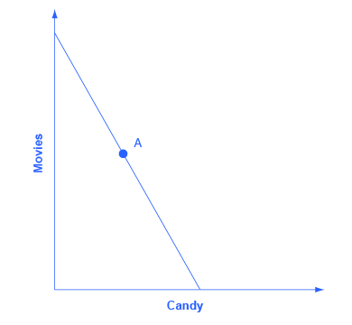
Step 1. Begin with a budget constraint showing the choice between two goods, which this example will call “candy” and “movies.” Choose a point A which will be the optimal choice, where the indifference curve will be tangent—but it is often easier not to draw in the indifference curve just yet. See [link] .
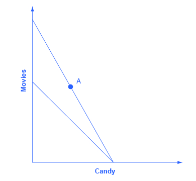
Step 2. Now the price of movies changes: let’s say that it rises. That shifts the budget set inward. You know that the higher price will push the decision-maker down to a lower level of utility, represented by a lower indifference curve. But at this stage, draw only the new budget set. See [link] .
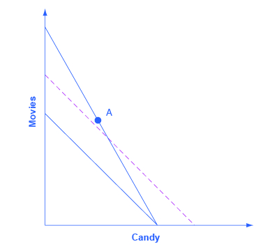
Step 3. The key tool in distinguishing between substitution and income effects is to insert a dashed line, parallel to the new budget line. This line is a graphical tool that allows you to distinguish between the two changes: (1) the effect on consumption of the two goods of the shift in prices—with the level of utility remaining unchanged—which is the substitution effect; and (2) the effect on consumption of the two goods of shifting from one indifference curve to the other—with relative prices staying unchanged—which is the income effect. The dashed line is inserted in this step. The trick is to have the dashed line travel close to the original choice A, but not directly through point A. See [link] .
Step 4. Now, draw the original indifference curve, so that it is tangent to both point A on the original budget line and to a point C on the dashed line. Many students find it easiest to first select the tangency point C where the original indifference curve touches the dashed line, and then to draw the original indifference curve through A and C. The substitution effect is illustrated by the movement along the original indifference curve as prices change but the level of utility holds constant, from A to C. As expected, the substitution effect leads to less consumed of the good that is relatively more expensive, as shown by the “s” (substitution) arrow on the vertical axis, and more consumed of the good that is relatively less expensive, as shown by the “s” arrow on the horizontal axis. See [link] .
Notification Switch
Would you like to follow the 'Principles of economics' conversation and receive update notifications?

|
|
|
|
|

|
|

|
|

|
|

|
|

|
|

|
|

|
|

|
|

|
|

|