

| << Chapter < Page | Chapter >> Page > |
The adverse selection of wage cuts argument points out that if an employer reacts to poor business conditions by reducing wages for all workers, then the best workers, those with the best employment alternatives at other firms, are the most likely to leave. The least attractive workers, with fewer employment alternatives, are more likely to stay. Consequently, firms are more likely to choose which workers should depart, through layoffs and firings, rather than trimming wages across the board. Sometimes companies that are going through tough times can persuade workers to take a pay cut for the short term, and still retain most of the firm’s workers. But these stories are notable because they are so uncommon. It is far more typical for companies to lay off some workers, rather than to cut wages for everyone.
The insider-outsider model of the labor force, in simple terms, argues that those already working for firms are “insiders,” while new employees, at least for a time, are “outsiders.” A firm depends on its insiders to grease the wheels of the organization, to be familiar with routine procedures, to train new employees, and so on. However, cutting wages will alienate the insiders and damage the firm’s productivity and prospects.
Finally, the relative wage coordination argument points out that even if most workers were hypothetically willing to see a decline in their own wages in bad economic times as long as everyone else also experiences such a decline, there is no obvious way for a decentralized economy to implement such a plan. Instead, workers confronted with the possibility of a wage cut will worry that other workers will not have such a wage cut, and so a wage cut means being worse off both in absolute terms and relative to others. As a result, workers fight hard against wage cuts.
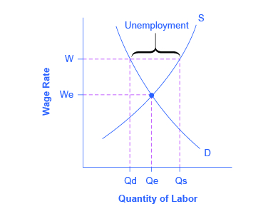
These theories of why wages tend not to move downward differ in their logic and their implications, and figuring out the strengths and weaknesses of each theory is an ongoing subject of research and controversy among economists. All tend to imply that wages will decline only very slowly, if at all, even when the economy or a business is having tough times. When wages are inflexible and unlikely to fall, then either short-run or long-run unemployment can result. This can be seen in [link] .
The interaction between shifts in labor demand and wages that are sticky downward are shown in [link] . [link] (a) illustrates the situation in which the demand for labor shifts to the right from D 0 to D 1 . In this case, the equilibrium wage rises from W 0 to W 1 and the equilibrium quantity of labor hired increases from Q 0 to Q 1 . It does not hurt employee morale at all for wages to rise.
[link] (b) shows the situation in which the demand for labor shifts to the left, from D 0 to D 1 , as it would tend to do in a recession. Because wages are sticky downward, they do not adjust toward what would have been the new equilibrium wage (Q 1 ), at least not in the short run. Instead, after the shift in the labor demand curve, the same quantity of workers is willing to work at that wage as before; however, the quantity of workers demanded at that wage has declined from the original equilibrium (Q 0 ) to Q 2 . The gap between the original equilibrium quantity (Q 0 ) and the new quantity demanded of labor (Q 2 ) represents workers who would be willing to work at the going wage but cannot find jobs. The gap represents the economic meaning of unemployment.
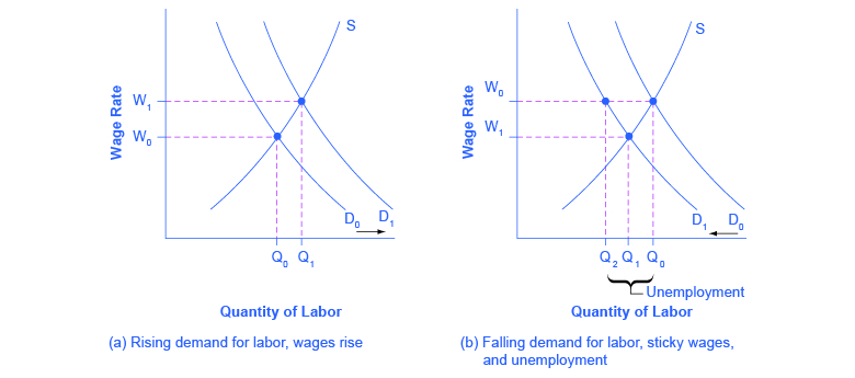
This analysis helps to explain the connection noted earlier: that unemployment tends to rise in recessions and to decline during expansions. The overall state of the economy shifts the labor demand curve and, combined with wages that are sticky downwards, unemployment changes. The rise in unemployment that occurs because of a recession is cyclical unemployment.
The St. Louis Federal Reserve Bank is the best resource for macroeconomic time series data, known as the Federal Reserve Economic Data (FRED). FRED provides complete data sets on various measures of the unemployment rate as well as the monthly Bureau of Labor Statistics report on the results of the household and employment surveys.
Cyclical unemployment rises and falls with the business cycle. In a labor market with flexible wages, wages will adjust in such a market so that quantity demanded of labor always equals the quantity supplied of labor at the equilibrium wage. Many theories have been proposed for why wages might not be flexible, but instead may adjust only in a “sticky” way, especially when it comes to downward adjustments: implicit contracts, efficiency wage theory, adverse selection of wage cuts, insider-outsider model, and relative wage coordination.
A government passes a family-friendly law that no companies can have evening, nighttime, or weekend hours, so that everyone can be home with their families during these times. Analyze the effect of this law using a demand and supply diagram for the labor market: first assuming that wages are flexible, and then assuming that wages are sticky downward.
Notification Switch
Would you like to follow the 'Principles of economics' conversation and receive update notifications?

|
|

|
|

|
|

|
|

|
|

|
|

|
|

|
|

|
|

|
|

|