

| << Chapter < Page | Chapter >> Page > |
This example suggests that the key factor is whether a firm can earn enough revenues to cover at least its variable costs by remaining open. Let’s return now to our raspberry farm. [link] illustrates this lesson by adding the average variable cost curve to the marginal cost and average cost curves. At a price of $2.20 per pack, as shown in [link] (a), the farm produces at a level of 50. It is making losses of $56 (as explained earlier), but price is above average variable cost and so the firm continues to operate. However, if the price declined to $1.80 per pack, as shown in [link] (b), and if the firm applied its rule of producing where P = MR = MC, it would produce a quantity of 40. This price is below average variable cost for this level of output. If the farmer cannot pay workers (the variable costs), then it has to shut down. At this price and output, total revenues would be $72 (quantity of 40 times price of $1.80) and total cost would be $144, for overall losses of $72. If the farm shuts down, it must pay only its fixed costs of $62, so shutting down is preferable to selling at a price of $1.80 per pack.
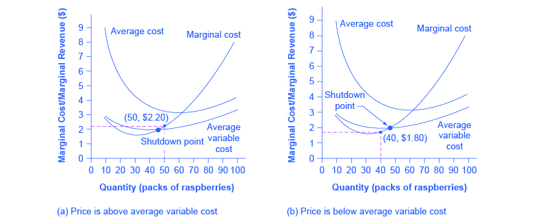
Looking at [link] , if the price falls below $2.05, the minimum average variable cost, the firm must shut down.
| Quantity | Total Cost | Fixed Cost | Variable Cost | Marginal Cost | Average Cost | Average Variable Cost |
|---|---|---|---|---|---|---|
| 0 | $62 | $62 | - | - | - | - |
| 10 | $90 | $62 | $28 | $2.80 | $9.00 | $2.80 |
| 20 | $110 | $62 | $48 | $2.00 | $5.50 | $2.40 |
| 30 | $126 | $62 | $64 | $1.60 | $4.20 | $2.13 |
| 40 | $144 | $62 | $82 | $1.80 | $3.60 | $2.05 |
| 50 | $166 | $62 | $104 | $2.20 | $3.32 | $2.08 |
| 60 | $192 | $62 | $130 | $2.60 | $3.20 | $2.16 |
| 70 | $224 | $62 | $162 | $3.20 | $3.20 | $2.31 |
| 80 | $264 | $62 | $202 | $4.00 | $3.30 | $2.52 |
| 90 | $324 | $62 | $262 | $6.00 | $3.60 | $2.91 |
| 100 | $404 | $62 | $342 | $8.00 | $4.04 | $3.42 |
The intersection of the average variable cost curve and the marginal cost curve, which shows the price where the firm would lack enough revenue to cover its variable costs, is called the shutdown point . If the perfectly competitive firm can charge a price above the shutdown point, then the firm is at least covering its average variable costs. It is also making enough revenue to cover at least a portion of fixed costs, so it should limp ahead even if it is making losses in the short run, since at least those losses will be smaller than if the firm shuts down immediately and incurs a loss equal to total fixed costs. However, if the firm is receiving a price below the price at the shutdown point, then the firm is not even covering its variable costs. In this case, staying open is making the firm’s losses larger, and it should shut down immediately. To summarize, if:
Notification Switch
Would you like to follow the 'Principles of economics' conversation and receive update notifications?

|
|
|
|
|

|
|

|
|

|
|

|
|

|
|

|
|

|
|

|
|

|
|

|