

| << Chapter < Page | Chapter >> Page > |
For simplicity, let's assume that the sampling frequency was one sample per second. This causes the sinusoid to have a period of 32 seconds and a frequency of 0.03125 cycles per second.
At a sampling rate of one sample per second, the folding frequency occurs at 0.5 cycles per second.
Dividing the folding frequency by 400 we conclude that the Fourier transform program computed a spectral value every 0.00125 cycles per second. Given thatevery second spectral value is zero, the zero values occur every 0.00250 cycles per second.
The top plot in Figure 14 shows the result of multiplying a cosine function having a frequency of 0.03125 cycles per second (the frequency of the sinusoid in the previous spectral analysis experiment) by a sine function having a frequency of 0.02875 cycles per second.
(This replicates one of the steps in the computation of the imaginary value in the Fourier transform).
| Figure 14. Average values of sinusoid products. |
|---|
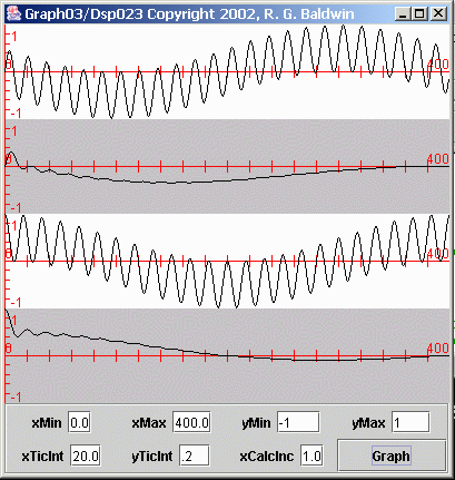 |
The difference between the frequencies of the cosine function and the sine function is 0.00250 cycles per second.
(Note that this frequency difference is the reciprocal of the actual number of samples in the earlier time series, which contained 400 samples.This is also the frequency interval on which the Fourier transform produced zero-valued points for the bottom plot in Figure 11 .)
The second plot in Figure 14 shows the average value of the time series in the first plot versus the number of samples included in the averaging window.
(This replicates another step in the computation of the imaginary value in the Fourier transform).
It is very important to note that this average plot goes to zero when 400 samples are included in the average.
Similarly, the third plot in Figure 14 shows the product of the same cosine function as above and another cosine function having the same frequency as thesine function described above.
(This replicates a step in the computation of the real value in the Fourier transform).
The fourth plot in Figure 14 shows the average value of the time series in the third plot.
(This replicates another step in the computation of the real value in the Fourier transform).
This average plot goes to zero at an averaging window of about 200 samples, and again at an averaging window of 400 samples.
The first point at which both average plots go to zero at the same point on the horizontal axis is at an averaging window of 400 samples.
(Both the real and imaginary values must go to zero in order for the spectral value produced by the Fourier transform to go to zero.)
Thus, the values produced by performing a Fourier transform on a single sinusoid go through zero at regular frequency intervals out from the peak inboth directions. The frequency intervals between the zero values are multiples of the reciprocal of the actual length of the sinusoid on which the transform isperformed.
Notification Switch
Would you like to follow the 'Digital signal processing - dsp' conversation and receive update notifications?

|
|

|
|

|
|

|
|

|
|

|
|
|
|
|

|
|

|
|

|