<< Chapter < Page Chapter >> Page >
A k = b = 0 M - 1 2 h ( n ) sin ( 2 π ( M - n ) k / N )

and

h ( n ) = 1 N [ k = 1 M 2 A k sin ( 2 π ( M - n ) k / N ) ]

Type 4. odd sampling

For Type 4 they are

A k = n = 0 N / 2 - 1 2 h ( n ) sin ( 2 π ( M - n ) k / N )

and

h ( n ) = 1 N [ k = 1 N / 2 - 1 2 A k sin ( 2 π ( M - n ) k / N ) + A N / 2 sin ( π ( M - n ) ) ] .

Type 3. even sampling

Using the frequency sampling scheme of [link] , the Type 3 equations become

A k = n = 0 M - 1 2 h ( n ) sin ( 2 π ( M - n ) ( k + 1 / 2 ) / N )

and

h ( n ) = 1 N [ k = 0 M - 1 2 A k sin ( 2 π ( M - n ) ( k + 1 / 2 ) / N ) ]

Type 4. even sampling

For Type 4 they are

A k = n = 0 N / 2 - 1 2 h ( n ) sin ( 2 π ( M - n ) ( k + 1 / 2 ) / N )

and

h ( n ) = 1 N [ k = 0 N / 2 - 1 2 A k sin ( 2 π ( M - n ) ( k + 1 / 2 ) / N ) ] .

These Type 3 and 4 formulas are useful in the design of differentiators and Hilbert transformers [1,2,9,31]directly and as the base of the discrete least-squared-error methods inthe section Discrete Frequency Samples of Error .

Frequency sampling design of fir filters by solution of simultaneous equations

A direct way of designing FIR filters from samples of a desired amplitude simply takes the sampled definition of the frequency response Equation 29 from FIR Digital Filters as

A ( ω k ) = n = 0 M - 1 2 h ( n ) cos ω k ( M - n ) + h ( M )

or the reduced form from Equation 37 from FIR Digital Filters as

A ( ω k ) = n = 0 M a ( n ) cos ( ω k ( M - n ) )

where

a ( n ) = { 2 h ( n ) for 0 n M - 1 h ( M ) for n = M 0 otherwise

for k=0,1,2,...,M and solves the M+1 simultaneous equations for a(n) or equivalently, h(n) . Indeed, this approach can be taken with general non-linear phase design from

Indeed, this approach can be taken with general non-linear phase design from

H ( ω k ) = n = 0 N - 1 h ( n ) e j ω k n

for k = 0 , 1 , 2 , , N - 1 which gives N equations with N unknowns.

This design by solving simultaneous equations allows non-equally spaced samples of the desired response. The disadvantage comes from the numericalcalculations taking considerable time and being subject to inaccuracies if the equations are ill-conditioned.

The frequency sampling design method is interesting but is seldom used for direct design of filters. It is sometimes used as an interpolatingmethod in other design procedures to find h ( n ) from calculated A ( ω k ) . It is also used as a basis for a least squares design method discussed inthe next section.

Examples of frequency sampling fir filter design

To show some of the characteristics of FIR filters designed by frequency sampling, we will design a Type 1., length-15 FIR low pass filter. Desired amplitude responsewas one in the pass band and zero in the stop band. The cutoff frequency was set at approximately f = 0 . 35 normalized. Using the formulas [link] , [link] , [link] , and [link] , we got impulse responses h ( n ) , which are use to generate the results shown in Figures  [link] and [link] .

The Type 1, length-15 filter impulse response is:

h 1 = - 0 . 5 0 1 . 1099 0 - 1 . 6039 0 4 . 494 7 4 . 494 0 - 1 . 6039 0 1 . 1099 0 - 0 . 5

The amplitude frequency response and zero locations are shown in [link] a

This image consist of 4 sets of parallel graphs. The left column of graphs are frequency responses and the right column of graphs are Zero locations. For all of the left column graphs the x axis is labeled Normalized Frequency and the y axis is labeled Amplitude Response, A. For all of the right column of graphs the x axis labeled the real part of z and the y axis is labeled the Imaginary part of z. The first Row of graphs is labeled Type 1. Frequency sample with odd spacing. The graph on the left consist of a right angle formed by a line extending from the y axis at 1 to the right where in intersects a line rising from the x axis at about .3. There is also a wave form with smaller hollow circles at points along it. This line begins at the same point as the line from the y axis. This line falls below the line from the y axis and then goes above it and the takes a more negative slope before reaching the right angle formed by the two lines. The line falls below the x axis and then archs above and below the axis until it runs off the graph. The first graph in the right column consists of  circle centered at the origin, with 10 smaller hollow circles around the left two-thirds of the circumference of the circle, two inside the circle on the inner right and two outside and to the right of the larger circle. The second row of graphs is very similar to the first row; these graphs are labeled Type 2.Frequency samples with odd spacing. The left graph is the same as the first in this column except that the line forming the right angle are a little smaller which in turn causes the waveform to reach the x axis a little earlier than the first graph. The graph in the right column looks exactly the same as the first one in the right column except that there are 11 hollow circle along the circumference of the circle. The third row of graphs is similar to the other graphs, but these are labeled Type 1. Frequency Sample with even spacing. The lines forming the right angle are a little larger and the waveform line starts above the line extending out from the y axis. Also once the wave intersects the x axis the wave amplitude is much less pronounced and almost looks like a straight line. The graph in the right column looks the same as the previous ones in the column except that there are only 9 hollow circles on the circumference of the circle. The graphs on the fourth and final row look exactly the same as the previous row, except that the organization of the hollow circles on the graph on the right is a little different. There are 11 hollow circles around the circumference of the larger circle. The middle three are tighly compressed together on the far left of the circumference whereas the remaining four on both the top and bottom are spread out at equal distances from one another.
Frequency Responses and Zero Locations of Length-15 and 16 FIR Filters Designed by Frequency Sampling

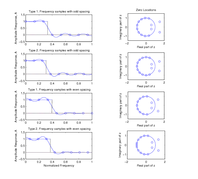
We see a good lowpass filter frequency response with the actual amplitude interpolating the desired values at 8 equally spaced points. Notice thereis considerable overshoot near the cutoff frequency. This is characteristic of frequency sampling designs and is a sort of “Gibbsphenomenon" but is even worse than that in a Fourier series expansion of a discontinuity. This Gibbs phenomenon could be reduced by using unequallyspaced samples and designing by solving simultaneous equations. Imagine sampling in the pass and stop bands of Figure 8c from FIR Digital Filters but not in the transitionband. The other responses and zero locations show theresults of different interpolation locations and lengths. Note the zero at -1 for the even filters.

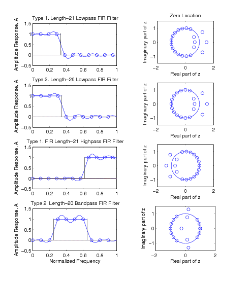
Examples of longer filters and of highpass and bandpass frequency sampling designs are shown in [link] . Note the difference of even and odd distributions of samples with with or without an interpolation pointat zero frequency. Note the results of different ideal filters and Type 1 or 2. Also note the relationship of the amplitude response and zerolocations.

This image consist of 4 sets of parallel graphs. The left column of graphs are frequency responses and the right column of graphs are Zero locations. For all of the left column graphs the x axis is labeled Normalized Frequency and the y axis is labeled Amplitude Response, A. For all of the right column of graphs the x axis labeled the real part of z and the y axis is labeled the Imaginary part of z. The first row of graphs are labeled Type 1. Length-21 Lowpass FIR Filter. The graph on the left hand column is comprised of a right angle formed by a line extending for the y axis at 1 to the right and another line extending up from the x axis at around .3. The waveform starts at (0,1) proceeding with a slight curve upward above the top line of the right angle and then curves under the line and again above the line. After this last curve the wave takes on a negative slope just before reaching the corner of the right angle. The line then progresses down to the y axis curves down and then undulates above and below the axis until the form runs off the graph. The graph in the right hand column is comprised of a circle centered around the origin 14 hollow circles around the left hand side of circumference of the larger circle, three hollow circles on the right inside area of the larger circle, and also three hollow circles to the right side outside the larger circle. The second row labeled Type 2. Length-20 Lowpass FIR Filter is very similar to the first row. The graph in the left column is exactly the same except that the lines creating the right angle are larger and thus the waveform proceeds a little bit earlier than the previous graph. The graph in the right column looks exactly the same except that there are only 13 small hollow circles around the circumference. The third row is labeled Type 1. FIR Length-21 Highpass FIR Filter is exactly the same as the previous two except that the graphs appear to be reversed horizontally. The fourth row of graphs is labeled Type 2. Length-20 Bandpass FIR Filter and is completely different from the previous graphs. The graph on the left hand side consists of a box formed by a two lines extending up from the x axis around .2 and .6 and then a line between the tops of these lines at 1. The waveform begins on the x axis undulating above and below the axis and then the waveform takes on a positive slope and restarts its undulation on the line between the two vertical lines and then the wave takes on a negative slope at the end of the line between the  vertical lines and the waveform then returns back to the x axis where the undulation above and below the axis. The graph on the right column is also completely different. There is a circle centered around the origin. On the circumference of this circle there are 7 small hollow circles on the left side and then 5 small hollow circles on the right side of the circumference. There is another hollow circle to the just to the left of the origin. There are also two hollow circles present on the inside of the larger circle. The bottom circle is at the bottom inside of the circle a little to the right of the x=0 and then there is another circle there on the top inside of the circle. Outside the circle there are also two circles, one above or below the larger circle. These circles are present to the right of x=0.
Frequency Response and Zero Locations of FIR Filters Designed by Frequency Sampling

Get Jobilize Job Search Mobile App in your pocket Now!

Get it on Google Play Download on the App Store Now


Source:  OpenStax, Digital signal processing and digital filter design (draft). OpenStax CNX. Nov 17, 2012 Download for free at http://cnx.org/content/col10598/1.6
Google Play and the Google Play logo are trademarks of Google Inc.

Notification Switch

Would you like to follow the 'Digital signal processing and digital filter design (draft)' conversation and receive update notifications?

Ask