

| << Chapter < Page | Chapter >> Page > |
At the same time, it is very difficult to convey very much information with a signal consisting of a continuous tone at a single frequency (other than the fact that the tone exists) . Communication systems designed to convey information usually encode that information by either turning the tone on and off or bycausing it to shift among a set of previously defined frequencies. The tone is often referred to as the carrier and the encoding of the information is often referred to as modulating the carrier.
Thus, you need greater bandwidth to reliably convey more information.
So far, we can draw one important conclusion from our experiment.
Shorter pulses require greater bandwidth.
This leads to an important question. What is the numerical relationship between pulse length and bandwidth? Although we can draw the above generalconclusion from Figure 2 , it is hard to draw any quantitative conclusions from Figure 2 . That brings us to the expanded plot of the spectral data shown in Figure 3 .
Figure 3 shows the left one-fourth of the spectral results from Figure 2 plotted in the same horizontal space. In other words, Figure 3 discards the upper three-fourths of the spectral results from Figure 2 and shows only the lower one-fourth of the spectral results on an expanded scale. Figure 3 also provides tick marks that make it convenient to perform measurements on theplots.
Also, whereas Figure 2 was plotted using the program named Graph06 , Figure 3 was plotted using the program named Graph03 . Thus, Figure 3 uses a different plotting format than Figure 2
| Figure 3. Expanded spectral analyses of five pulses. |
|---|
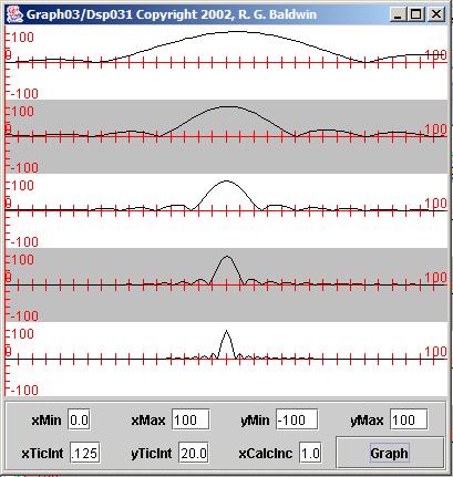 |
The curves in Figure 3 are spread out to the point that we can pick some approximate numeric values off the plot, and from this, we can draw a verysignificant conclusion.
For purposes of our approximation, consider the bandwidth to be the distance along the frequency axis between the points where the curves touch zero oneither side of the peak. Using this approximation, the bandwidth indicated by the spectral analyses in Figure 3 shows the bandwidth of each spectrum to be twice as wide as the one below it.
Referring back to Figure 1 , recall that the length of each pulse was half that of the one below it. The conclusion is:
The bandwidth of a truncated sinusoidal pulse is inversely proportional to the length of the pulse.
If you reduce the length of the pulse by a factor of two, you must double thebandwidth of a transmission system designed to reliably transmit a pulse of that length.
This will also be an important conclusion regarding our ability to separate and identify the two spectral peaks in the burst of acoustic energy described inour original hypothetical situation .
The generation of the signals and the spectral analysis for the results presented in Figure 2 and Figure 3 were performed using the program named Dsp031 . A complete listing of the program is shown in Listing 10 near the end of the module.
Notification Switch
Would you like to follow the 'Digital signal processing - dsp' conversation and receive update notifications?

|
|

|
|

|
|

|
|

|
|

|
|

|
|

|
|

|
|

|