

| << Chapter < Page | Chapter >> Page > |
| Figure 1. Required parameters. |
|---|
Data length as type int
Number of sinusoids as type int.  Max value is 5.List of sinusoid frequency values as type double.
List of sinusoid amplitude values as type double. |
The number of values in each of the lists must match the value for the number of sinusoids. Also, you must not allow blank lines at the end of the data in thefile.
Each frequency value is specified as a type double value representing a fractional part of the sampling frequency.
(For example, a double value of 0.5 specifies one-half the sampling frequency, or the Nyquist folding frequency. A double value of 2.0 specifiesa frequency that is twice the sampling frequency.)
Figure 2 shows the contents of the file named Dsp029.txt that I used to produce the output shown in Figure 3 . I will discuss that output later.
| Figure 2. Actual parameter values. |
|---|
50.0
50.03125
0.06250.125
0.250.5
9090
9090
90 |
The plotting program that is used to plot the output data from this program requires that the program implement GraphIntfc01 . I discussed that interface in the module titled Plotting Engineering and Scientific Data using Java . For example, the plotting program named Graph06 can be used to plot the data produced by this program. When it is used, the program is executed and its output is plotted byentering the following at the command line prompt:
java Graph06 Dsp029
Figure 3 shows the output produced by running the program named Dsp029 with the parameters shown in Figure 2 and then adjusting the xMax parameter in thetextbox at the bottom of the display.
| Figure 3. Program output for five sinusoids. |
|---|
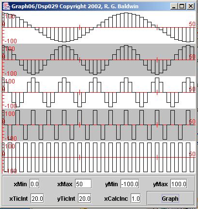 |
Each of the five horizontal plots in Figure 3 shows a sampled sinusoid. Each of the vertical bars represents one sample value for a given sinusoid.
If you examine the frequency values in Figure 2 carefully, you will see that they represent the sampling frequency divided by the factors 32, 16, 8, 4, and2. Thus, the last frequency value is the Nyquist folding frequency and the first four frequency values are related to that frequency by multiples of two.
The horizontal plot at the top of Figure 3 is a reasonably well defined cosine wave. The horizontal plot at the bottom of Figure 3 shows the result of having exactly two samples per cycle of the sinusoid. Using this plottingscheme, the sampled sinusoid is represented as a square wave. Using another plotting scheme (such as that used in the program named Graph03 ) the sampled sinusoid at the bottom would be represented as a triangular wave.
Regardless of the plotting scheme used, it should be obvious that a set of uniform samples cannot possibly represent frequencies higher than one-half thesampling frequency because then there would be less than one sample per cycle of the sinusoid.
Now I will show you why the frequency at one-half the sampling frequency is referred to as the folding frequency using the new set of frequency values shownin Figure 4 .
Notification Switch
Would you like to follow the 'Digital signal processing - dsp' conversation and receive update notifications?

|
|

|
|

|
|

|
|

|
|

|
|
|
|
|

|
|

|
|

|