0.6 Probably approximately correct (pac) learning  (Page 2/2)

Data adaptive model spaces

Structural risk minimization (srm)

The basic idea is to select ${\mathcal{F}}_n$ based on the training data themselves. Let ${\mathcal{F}}_1$ , ${\mathcal{F}}_2$ , ...be a sequence of model spaces of increasing sizes/complexities with

Let

be a function from ${\mathcal{F}}_k$ that minimizes the empirical risk. This gives us a sequence of selected models ${\widehat{f}}_{n,1},{\widehat{f}}_{n,2},\cdots$ Also associate with each set ${\mathcal{F}}_k$ a value $C_{n,k}>0$ that measures the complexity or “size” of the set ${\mathcal{F}}_k$ . Typically, $C_{n,k}$ is monotonically increasing with $k$ (since the sets are of increasing complexity) and decreasing with $n$ (since we become more confident with more training data). More precisely, suppose thatthe $C_{n,k}$ chosen so that

for some small $\delta >0$ . Then we may conclude that with very high probability (at least $1-\delta$ ) the empirical risk ${\widehat{R}}_n$ is within $C_{n,k}$ of $R$ uniformly on the class ${\mathcal{F}}_k$ . This type of bound suffices to bound the estimation error (variance)of the model selection process of the form $R\left(f\right)\le {\widehat{R}}_n\left(f\right)+C_{n,k}$ , and SRM selects the final model by minimizing this bound over all functions in ${\bigcup }_{k\ge 1}{\mathcal{F}}_k$ . The selected model is given by ${\widehat{f}}_{n,\widehat{k}}$ , where

A typical example could be the use of VC dimension to characterize the complexity of the collectionof model spaces i.e., $C_{n,k}$ is derived from a bound on the estimation error.

Complexity regularization

Consider a very large class of candidate models $\mathcal{F}$ . To each $f\in \mathcal{F}$ assign a complexity value $C_n\left(f\right)$ . Assume that the complexity value is chosen so that

This probability bound also implies an upper bound on the estimation error and complexity regularization is based on the criterion

Complexity Regularization and SRM are very similar and equivalent in certain instances. A distinguishing feature of SRM and complexityreqularization techniques is that the complexity and structure of the model is not fixed prior to examining the data; the data aid in theselection of the best complexity. In fact, the key difference compared to the Method of Sieves is that these techniques can allow the data toplay an integral role in deciding where and how to average the data.

Probably approximately correct (pac) learning

Probability bounds of the forms in [link] and [link] are the foundation for SRM and complexity regularization techniques.The simplest of these bounds are known as PAC bounds in the machine learning community.

Approximation and estimation errors

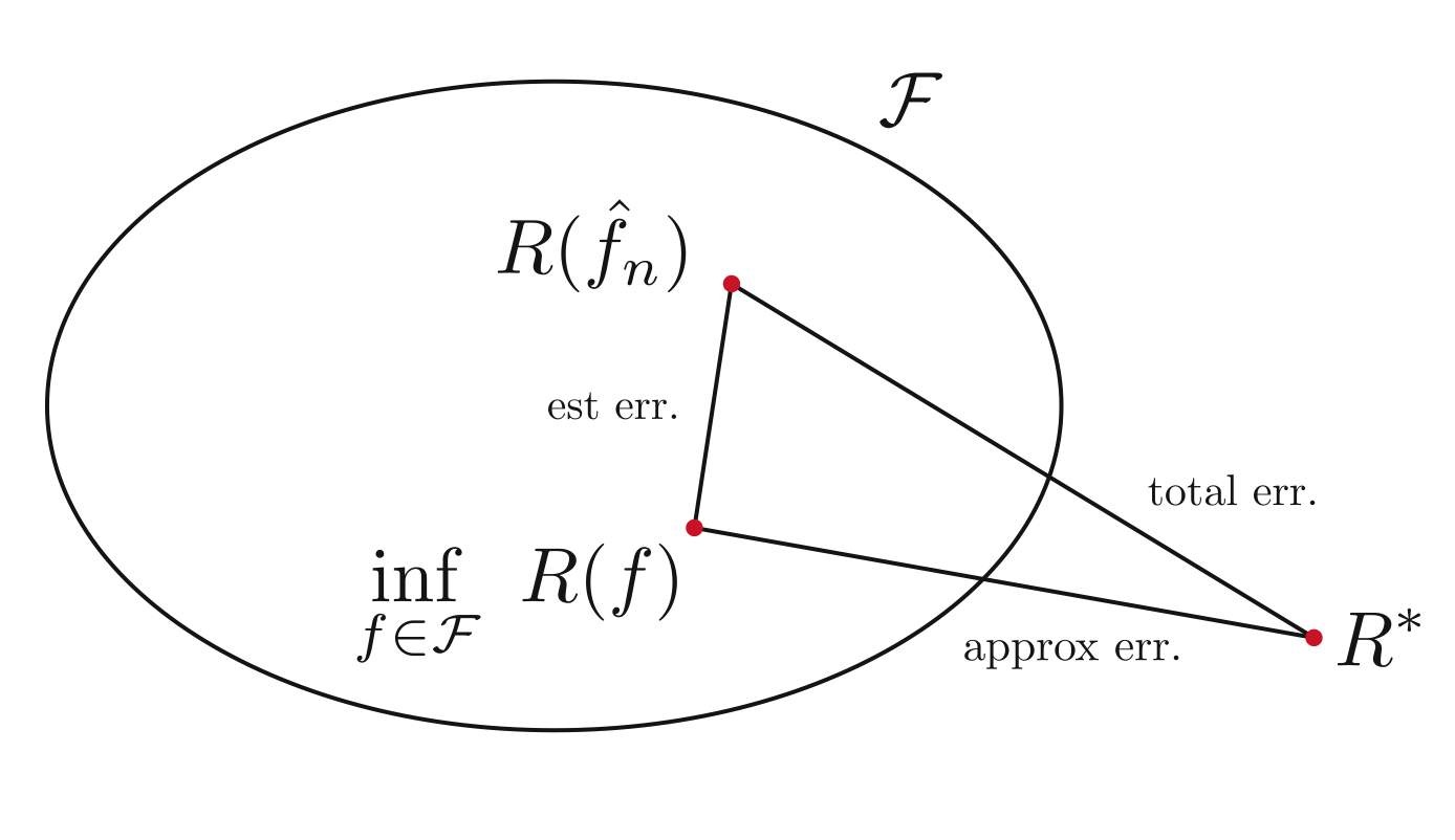
In order to develop complexity regularization schemes we will need to revisit the estimation error / approximation error trade-off. Let ${\widehat{f}}_n=arg{min}_{f\in \mathcal{F}}{\widehat{R}}_n\left(f\right)$ for some space of models $\mathcal{F}$ .

The approximation error depends on how close $f^{*}$ is close to $\mathcal{F}$ , and without making assumptions, this is unknown. The estimation error isquantifiable, and depends on the complexity or size of $\mathcal{F}$ . The error decomposition is illustrated in [link] . The estimation error quantifies how much we can “trust” the empiricalrisk minimization process to select a model close to the best in a given class.

Probability bounds of the forms in [link] and [link] guarantee that the empirical risk is uniformly close to the true risk, and using [link] and [link] it is possible to show that with high probability the selected model ${\widehat{f}}_n$ satisfies

or

The pac learning model

The estimation error will be small if $R\left({\widehat{f}}_n\right)$ is close to ${inf}_{f\in \mathcal{F}}R\left(f\right)$ . PAC learning expresses this as follows. We want ${\widehat{f}}_n$ to be a “probably approximately correct” (PAC) model from $\mathcal{F}$ . Formally, we say that ${\widehat{f}}_n$ is $\epsilon$ accurate with confidence $1-\delta$ , or $(\epsilon ,\delta )-$ PAC for short, if

This says that the difference between $R\left({\widehat{f}}_n\right)$ and ${inf}_{f\in \mathcal{F}}R\left(f\right)$ is greater than $\epsilon$ with probability less than $\delta$ . Sometimes, especially in the machine learning community, PAC bounds are stated as, “with probability of at least $1-\delta$ , $|R\left({\widehat{f}}_n\right)-{inf}_{f\in \mathcal{F}}R\left(f\right)|\le \epsilon$ ”

To introduce PAC bounds, let us consider a simple case. Let $\mathcal{F}$ consist of a finite number of models, and let $\left|\mathcal{F}\right|$ denote that number. Furthermore, assume that ${min}_{f\in \mathcal{F}}R\left(f\right)=0$ .

Assume $\left|\mathcal{F}\right|<\infty$ and ${min}_{f\in \mathcal{F}}R\left(f\right)=0$ , where $R\left(f\right)=P\left(f\right(X)\ne Y)$ . Let ${\widehat{f}}_n=arg{min}_{f\in \mathcal{F}}{\widehat{R}}_n\left(f\right)$ , where ${\widehat{R}}_n\left(f\right)=\frac{1}{n}{\sum }_{i=1}^n{\mathbf{1}}_{\{f\left(X_i\right)\ne Y_i\}}$ . Then for every $n$ and $\epsilon >0$ ,

Since ${min}_{f\in \mathcal{F}}R\left(f\right)=0$ , it follows that ${\widehat{R}}_n\left({\widehat{f}}_n\right)=0$ . In fact, there may be several $f\in \mathcal{F}$ such that ${\widehat{R}}_n\left(f\right)=0$ . Let $\mathcal{G}=\{f:{\widehat{R}}_n\left(f\right)=0\}$ .

The last inequality follows from the fact that if $R\left(f\right)=P\left(f\right(X)\ne Y)>\epsilon$ , then the probability that $n$ i.i.d. samples will satisfy $f\left(X\right)=Y$ is less than or equal to ${(1-\epsilon )}^n$ . Note that this is simply the probability that ${\widehat{R}}_n\left(f\right)=\frac{1}{n}{\sum }_{i=1}^n{\mathbf{1}}_{\{f\left(X_i\right)\ne Y_i\}}=0$ . Finally apply the inequality $1-x\le e^{-x}$ to obtain the desired result.

Note that for $n$ sufficiently large, $\delta =\left|\mathcal{F}\right|e^{-n\epsilon }$ is arbitrarily small. To achieve a $(\epsilon ,\delta )$ -PAC bound for a desired $\epsilon >0$ and $\delta >0$ we require at least $n=\frac{log\left|\mathcal{F}\right|-log\delta }{\epsilon }$ training examples.

Assume that $\left|\mathcal{F}\right|<\infty$ and ${min}_{f\in \mathcal{F}}R\left(f\right)=0$ . Then for every $n$

Recall that for any non-negative random variable $Z$ with finite mean, $E\left[Z\right]={\int }_0^{\infty }P(Z>t)dt$ . This follows from an application of integration by parts.

Minimizing with respect to $u$ produces the smallest upper bound with $u=\frac{log\left|\mathcal{F}\right|}{n}$