

| << Chapter < Page | Chapter >> Page > |
This method accepts an incoming complex sample value and the position in the series associated with that sample. The method corrects the real and imaginarytransform values for that complex sample to reflect the specified position in the input series.
After correcting the transform values for the sample on the basis of position, the method updates the corresponding real and imaginary valuescontained in array objects that are used to accumulate the real and imaginary values for all of the samples.
References to the array objects are received as input parameters. Outgoing results are scaled by an incoming parameter in an attempt to cause the outputvalues to fall within a reasonable range in case someone wants to plot them.
The incoming parameter named length specifies the number of output samples that are to be produced.
Hopefully this explanation will make it possible for you to understand the code in Listing 4 .
Note in particular the use of the Math.cos and Math.sin methods to apply the cosine and sine curves in the correction of the transforms of the individual complex samples. This is used to produceresults similar to those shown in Figure 5 through Figure 7 .
A real FFT program would probably compute the cosine and sine values only once, put them in a table and extract them from the table when needed.
Note the use of the position and length parameters in the computation of the angle that is passed as an argument to the Math.cos and Math.sin methods.
Also note how the correction is made separately on the real and imaginary parts of the input. This produces results similar to those shown in Figure 7 after those results are added in the accumulators.
Returning now to the main method, the code in Listing 5 prepares the input data and the output arrays for the first case that we will look at. This case islabeled as Case A.
| Listing 5. The remainder of the main method. |
|---|
System.out.println("Case A");
    double[]realInA =
               {0,1,0,0,0,0,0,0,0,0,0,0,0,0,0,1};double[] imagInA ={0,0,0,0,0,0,0,0,0,0,0,0,0,0,0,0};

    double[]realOutA = new double[16];double[] imagOutA = new double[16];

    //Perform the transform and display the// transformed results for the original
    // complex series.transform.doIt(realInA,imagInA,2.0,realOutA,
imagOutA);display(realOutA,imagOutA); |
Note that for Case A, the input complex series contains non-zero values only in the real part. Also, most of the values in the real part are zero.
Case A is shown in graphic form in Figure 9 . As you can see, the input series consists of two non-zero values in the real part. All the values in theimaginary part are zero.
| Figure 9. Case A. Transform of a real sample with two non-zero values. |
|---|
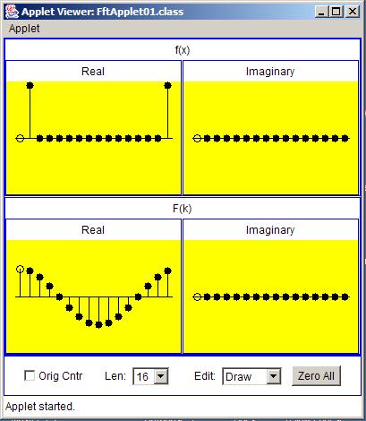 |
The real part of the transform of the complex input series looks like one cycle of a cosine curve. All of the values in the imaginary part of thetransform result are zero.
As you saw in Listing 5 , the code in the main method calls a method named display to display the complex transform output in numeric form on the screen. The output produced by Listing 5 is shown in Figure 10 . (Note that I manually inserted line breaks to force the material to fit in this narrowpublication format.)
Notification Switch
Would you like to follow the 'Digital signal processing - dsp' conversation and receive update notifications?

|
|

|
|

|
|

|
|

|
|

|
|

|
|

|
|
|
|
|

|