

| << Chapter < Page | Chapter >> Page > |
During the 1960s, the Phillips curve was seen as a policy menu. A nation could choose low inflation and high unemployment, or high inflation and low unemployment, or anywhere in between. Fiscal and monetary policy could be used to move up or down the Phillips curve as desired. Then a curious thing happened. When policymakers tried to exploit the tradeoff between inflation and unemployment, the result was an increase in both inflation and unemployment. What had happened? The Phillips curve shifted.
The U.S. economy experienced this pattern in the deep recession from 1973 to 1975, and again in back-to-back recessions from 1980 to 1982. Many nations around the world saw similar increases in unemployment and inflation. This pattern became known as stagflation . (Recall from The Aggregate Demand/Aggregate Supply Model that stagflation is an unhealthy combination of high unemployment and high inflation.) Perhaps most important, stagflation was a phenomenon that could not be explained by traditional Keynesian economics.
Economists have concluded that two factors cause the Phillips curve to shift. The first is supply shocks, like the Oil Crisis of the mid-1970s, which first brought stagflation into our vocabulary. The second is changes in people’s expectations about inflation. In other words, there may be a tradeoff between inflation and unemployment when people expect no inflation, but when they realize inflation is occurring, the tradeoff disappears. Both factors (supply shocks and changes in inflationary expectations) cause the aggregate supply curve, and thus the Phillips curve, to shift.
In short, a downward-sloping Phillips curve should be interpreted as valid for short-run periods of several years, but over longer periods, when aggregate supply shifts, the downward-sloping Phillips curve can shift so that unemployment and inflation are both higher (as in the 1970s and early 1980s) or both lower (as in the early 1990s or first decade of the 2000s).
Keynesian macroeconomics argues that the solution to a recession is expansionary fiscal policy , such as tax cuts to stimulate consumption and investment, or direct increases in government spending that would shift the aggregate demand curve to the right. For example, if aggregate demand was originally at ADr in [link] , so that the economy was in recession, the appropriate policy would be for government to shift aggregate demand to the right from ADr to ADf, where the economy would be at potential GDP and full employment.
Keynes noted that while it would be nice if the government could spend additional money on housing, roads, and other amenities, he also argued that if the government could not agree on how to spend money in practical ways, then it could spend in impractical ways. For example, Keynes suggested building monuments, like a modern equivalent of the Egyptian pyramids. He proposed that the government could bury money underground, and let mining companies get started to dig the money up again. These suggestions were slightly tongue-in-cheek, but their purpose was to emphasize that a Great Depression is no time to quibble over the specifics of government spending programs and tax cuts when the goal should be to pump up aggregate demand by enough to lift the economy to potential GDP .
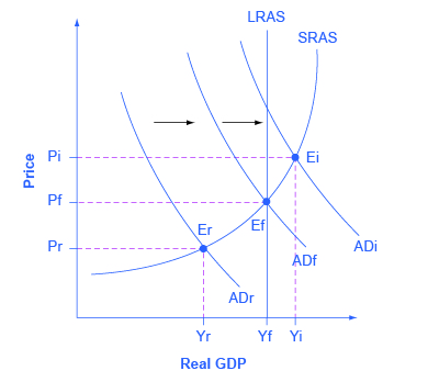
The other side of Keynesian policy occurs when the economy is operating above potential GDP. In this situation, unemployment is low, but inflationary rises in the price level are a concern. The Keynesian response would be contractionary fiscal policy , using tax increases or government spending cuts to shift AD to the left. The result would be downward pressure on the price level, but very little reduction in output or very little rise in unemployment. If aggregate demand was originally at ADi in [link] , so that the economy was experiencing inflationary rises in the price level, the appropriate policy would be for government to shift aggregate demand to the left, from ADi toward ADf, which reduces the pressure for a higher price level while the economy remains at full employment.
In the Keynesian economic model, too little aggregate demand brings unemployment and too much brings inflation. Thus, you can think of Keynesian economics as pursuing a “Goldilocks” level of aggregate demand: not too much, not too little, but looking for what is just right.
A Phillips curve shows the tradeoff between unemployment and inflation in an economy. From a Keynesian viewpoint, the Phillips curve should slope down so that higher unemployment means lower inflation, and vice versa. However, a downward-sloping Phillips curve is a short-term relationship that may shift after a few years.
Keynesian macroeconomics argues that the solution to a recession is expansionary fiscal policy, such as tax cuts to stimulate consumption and investment, or direct increases in government spending that would shift the aggregate demand curve to the right. The other side of Keynesian policy occurs when the economy is operating above potential GDP. In this situation, unemployment is low, but inflationary rises in the price level are a concern. The Keynesian response would be contractionary fiscal policy, using tax increases or government spending cuts to shift AD to the left.
Hoover, Kevin. “Phillips Curve.” The Concise Encyclopedia of Economics . http://www.econlib.org/library/Enc/PhillipsCurve.html.
U.S. Government Printing Office. “Economic Report of the President.” http://1.usa.gov/1c3psdL.
Notification Switch
Would you like to follow the 'Macroeconomics' conversation and receive update notifications?

|
|
|
|
|

|
|

|
|
|
|
|

|
|

|
|

|
|

|
|

|
|

|
|

|