

| << Chapter < Page | Chapter >> Page > |
The special case for is not of lowest order. It can be factored into [link] squared. Any length-4 even-symmetric filter can be factored intoproducts of terms of the form of [link] and [link] .
The fourth case is of an even-symmetric length-5 filter of the form
For and , the zeros are neither real nor on the unit circle; therefore, they must have complex conjugatesand have images about the unit circle. The form of the transfer function is
If one of the zeros of a length-5 filter is on the real axis or on the unit circle, can be factored into a product of lower order terms of the forms in [link] , [link] , and [link] and, therefore, is not of lowest order. The odd symmetric filters of [link] are described by the above factors plus the basic length-2 filter described by
The zero locations for the four basic cases of Type 1 and 2 FIR filters are shown in [link] . The locations for the Type 3 and 4 odd-symmetric cases of [link] are the same, plus the zero at one from [link] .
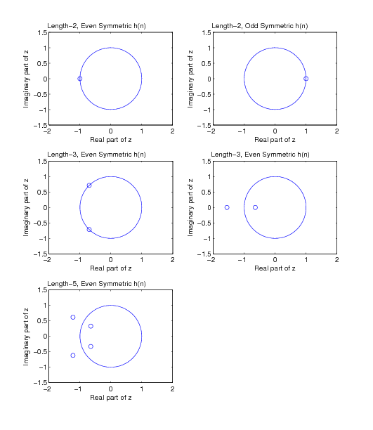
From this analysis, it can be concluded that all linear-phase FIR filters have zeros either on the unit circle or in thereciprocal symmetry of [link] or [link] about the unit circle, and their transfer functionscan always be factored into products of terms with these four basic forms. This factored form can beused in implementing a filter by cascading short filters to realize a long filter. Knowledge of the locations of the transferfunction zeros helps in developing filter design and analysis programs. Notice how these zero locations are consistent withthe amplitude responses illustrated in [link] and [link] .
In this section the basic characteristics of the FIR filter have been derived. For the linear-phase case, the frequencyresponse can be calculated very easily. The effects of the linear phase can be separated so that the amplitude can be approximatedas a real-valued function. This is a very useful property for filter design. It was shown that there are four basic types oflinear-phase FIR filters, each with characteristics that are also important for design. The frequency response can be calculatedby application of the DFT to the filter coefficients or, for greater resolution, to the filter coefficients with zeros added to increase the length. A very efficient calculation of the DFTuses the Fast Fourier Transform (FFT). The frequency response can also be calculated by special formulas that include the effectsof linear phase.
Because of the linear-phase requirements, the zeros of the transfer function must lie on the unit circle in the z plane oroccur in reciprocal pairs around the unit circle. This gives insight into the effects of the zero locations on the frequencyresponse and can be used in the implementation of the filter.
The FIR filter is very attractive from several points of view. It alone can achieve exactly linear phase. It is easilydesigned using methods that are linear. The filter cannot be unstable. The implementation or realization in hardware or on acomputer is basically the calculation of an inner product, which can be accomplished very efficiently. On the negative side, theFIR filter may require a rather long length to achieve certain frequency responses. This means a large number of arithmeticoperations per output value and a large number of coefficients that have to be stored. The linear-phase characteristic makes thetime delay of the filter equal to half its length, which may be large.
How the FIR filter is implemented and whether it is chosen over alternatives depends strongly on the hardware or computer to beused. If an array processor is used, an FFT implementation [link] would probably be selected. If a fixed point TMS320 signal processor is used, a direct calculation of the inner product is probably best. Ifa floating point DSP or microprocessor with floating-point arithmetic is used, an IIR filter may be chosen over the FIR, or theimplementation of the FIR might take into account the symmetries of the filter coefficients to reduce arithmetic. To make these choices,the characteristics developed in this chapter, together with the results developed later in these notes, must be considered.
A central characteristic of engineering is design. Basic to DSP is the design of digital filters. In many cases, the specifications ofa design is given in the frequency domain and the evaluation of the design is often done in the frequency domain. A typical sequence ofsteps in design might be:
This approach is often used iteratively. After the best filter is designed and evaluated, the desired response and/or the allowedclass and/or the measure of quality might be changed; then the filter would be redesigned and reevaluated.
The ideal response of a lowpass filter is given in [link] .
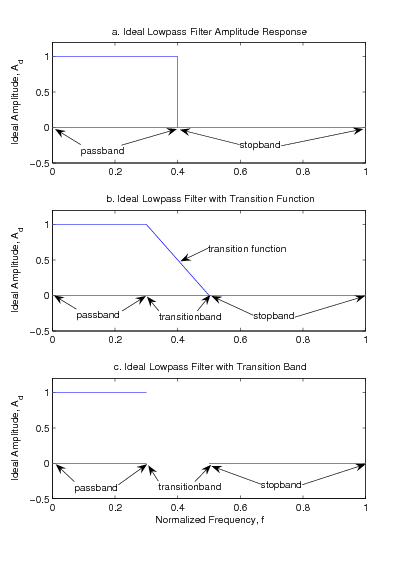
[link] a is the basic lowpass response that exactly passes frequencies from zero up to a certain frequency, then rejects(multiplies those frequency components by zero)the frequencies above that. [link] b introduces a “transitionband" between the pass and stopband to make the design easier and more efficient. [link] c introducess a transitionband which is not used in the approximation of the actual to the ideal responses. Each ofthese ideal responses (or other similar ones) will fit a particular application best.
Notification Switch
Would you like to follow the 'Digital signal processing and digital filter design (draft)' conversation and receive update notifications?

|
|

|
|

|
|

|
|

|
|
|
|
|

|
|
|
|
|
|
|
|

|