

| << Chapter < Page | Chapter >> Page > |
The flow of an ideal fluid (inviscid and incompressible) in two dimensions can be calculated for many configurations through the use of potential flow and complex variables. At a solid boundary, the ideal fluid has zero flux (the normal component of velocity is equal to that of the solid) but the tangential velocity may not be equal to that of the solid. Real fluids have a finite viscosity and (with only a few exceptions) the tangential component of velocity is equal to that of the solid, i.e., the boundary condition of no-slip. In many cases, the "external flow" sufficiently far from a solid body can be modeled as that of an ideal fluid and the effect of finite viscosity effects the flow only near the surface of the body (and downstream of the body). These situations can be treated by application of the boundary layer theory.
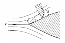
The underlying assumption in the boundary layer theory is that there is a very thin layer near the body where the gradient of the tangential velocity is very large due to the action of viscosity and the no-slip boundary condition. Elsewhere the effect of viscosity is assumed to be unimportant and can be modeled as inviscid or potential flow.
The continuity equation and equations of motion were specialized in Chapter 6 with the assumption that the boundary layer thickness, , is small compared to the characteristic dimension of the body, , i.e., . The equations (known as Prandtl's boundary layer equations) and boundary conditions are recalled here.
The remaining terms in the equation of motion and continuity equation are of similar magnitude if
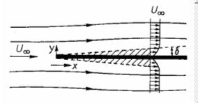
The assumption that the boundary layer thickness is small compared to the characteristic length of the body requires that the Reynolds number be large compared to unity if the terms in the equation of motion are to be of similar magnitude. If is to represent the distance, , from the leading edge of the boundary layer, the above relation describes the thickness of the boundary layer as a function of distance from the leading edge.
Another quantity that is of interest in boundary layer theory is the local drag coefficient due to the wall shear stress (some definitions differ by a factor of 2). The mean drag coefficient is the average value of this quantity over the surface of the body.
Notification Switch
Would you like to follow the 'Transport phenomena' conversation and receive update notifications?

|
|

|
|

|
|

|
|

|
|

|
|

|
|

|
|

|
|

|