

| << Chapter < Page | Chapter >> Page > |
The appearance of the investment function as a horizontal line does not mean that the level of investment never moves. It means only that in the context of this two-dimensional diagram, the level of investment on the vertical aggregate expenditure axis does not vary according to the current level of real GDP on the horizontal axis. However, all the other factors that vary investment—new technological opportunities, expectations about near-term economic growth, interest rates, the price of key inputs, and tax incentives for investment—can cause the horizontal investment function to shift up or down.
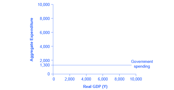
In the Keynesian cross diagram, government spending appears as a horizontal line, as in [link] , where government spending is set at a level of 1,300. As in the case of investment spending, this horizontal line does not mean that government spending is unchanging. It means only that government spending changes when Congress decides on a change in the budget, rather than shifting in a predictable way with the current size of the real GDP shown on the horizontal axis.
The situation of taxes is different because taxes often rise or fall with the volume of economic activity. For example, income taxes are based on the level of income earned and sales taxes are based on the amount of sales made, and both income and sales tend to be higher when the economy is growing and lower when the economy is in a recession. For the purposes of constructing the basic Keynesian cross diagram, it is helpful to view taxes as a proportionate share of GDP. In the United States, for example, taking federal, state, and local taxes together, government typically collects about 30–35 % of income as taxes.
[link] revises the earlier table on the consumption function so that it takes taxes into account. The first column shows national income. The second column calculates taxes, which in this example are set at a rate of 30%, or 0.3. The third column shows after-tax income; that is, total income minus taxes. The fourth column then calculates consumption in the same manner as before: multiply after-tax income by 0.8, representing the marginal propensity to consume, and then add $600, for the amount that would be consumed even if income was zero. When taxes are included, the marginal propensity to consume is reduced by the amount of the tax rate, so each additional dollar of income results in a smaller increase in consumption than before taxes. For this reason, the consumption function, with taxes included, is flatter than the consumption function without taxes, as [link] shows.
Notification Switch
Would you like to follow the 'Principles of macroeconomics for ap® courses' conversation and receive update notifications?

|
|
|
|
|

|
|

|
|

|
|

|
|

|
|

|
|

|
|
|
|
|
|
|
|

|