This module describes the continuous time Fourier Series (CTFS).
It is based on the following modules:Fourier Series: Eigenfunction Approach at http://cnx.org/content/m10496/latest/ by Justin Romberg,
Derivation of Fourier Coefficients Equation at http://cnx.org/content/m10733/latest/ by Michael Haag,Fourier Series and LTI Systems at http://cnx.org/content/m10752/latest/ by Justin Romberg, and
Fourier Series Wrap-Up at http://cnx.org/content/m10749/latest/ by Michael Haag and Justin Romberg.
Introduction
In this module, we will derive an expansion for
continuous-time, periodic functions, and in doing so, derive the
Continuous Time Fourier Series (CTFS).
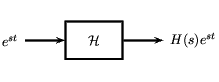
Since
complex
exponentials are
eigenfunctions of linear time-invariant (LTI)
systems , calculating the output of an LTI system
given
as an input amounts to simple multiplication, where
is the eigenvalue corresponding to s. As shown in the figure, a simple exponential input would yield the output
Simple LTI system.
Using this and the fact that
is linear, calculating
for combinations of complex exponentials is also
straightforward.
The action of
on an input such
as those in the two equations above is easy to explain.
independently
scales each exponential component
by a different complex number
. As such, if we can write a function
as a combination of complex exponentials it allows us to easily calculate the output of a system.
Fourier series synthesis
Joseph
Fourier demonstrated that an arbitrary
can be written as a linear combination of harmonic
complex sinusoids
where
is the fundamental frequency. For almost all
of practical interest, there exists
to make
[link] true. If
is finite energy (
), then the equality in
[link] holds in the sense of energy convergence; if
is continuous, then
[link] holds
pointwise. Also, if
meets some mild conditions (the Dirichlet
conditions), then
[link] holds
pointwise everywhere except at points of discontinuity.
The
- called the Fourier coefficients -
tell us "how much" of the sinusoid
is in
.
The formula shows
as a sum of complex exponentials, each of which is easily processed by an
LTI system (since it is an eigenfunction of
every LTI system). Mathematically,
it tells us that the set ofcomplex exponentials
form a basis for the space of T-periodic continuous
time functions.
Interact(when online) with a Mathematica CDF demonstrating sinusoid synthesis. To download, right click and save as .cdf.
Guitar oscillations on an iphone
Fourier series analysis
Finding the coefficients of the Fourier series expansion involves some algebraic manipulation of the synthesis formula.
First of all we will multiply both sides of the equation by
, where
.
Now integrate both sides over a given period,
:
On the right-hand side we can switch the summation andintegral and factor the constant out of the
integral.
Now that we have made this seemingly more complicated, let us
focus on just the integral,
, on the right-hand side of the above equation.
For this integral we will need to consider two cases:
and
. For
we will have:
For
, we will have:
But
has an integer number of periods,
, between
and
. Imagine a graph of the
cosine; because it has an integer number of periods, there areequal areas above and below the x-axis of the graph. This
statement holds true for
as well. What this means is
which also holds for the integral involving the sine function.
Therefore, we conclude the following about our integral ofinterest:
Now let us return our attention to our complicated equation,
[link] , to see if we can finish
finding an equation for our Fourier coefficients. Using thefacts that we have just proven above, we can see that the only
time
[link] will have a nonzero
result is when
and
are equal:
Finally, we have our general equation for the Fourier
coefficients:
Consider the square wave function given by
on the unit interval
.
Thus, the Fourier coefficients of this function found using the Fourier series analysis formula are
Because complex exponentials are eigenfunctions of LTI systems, it is often useful to represent signals using a set of complex exponentials as a basis. The continuous time Fourier series synthesis formula expresses a continuous time, periodic function as the sum of continuous time, discrete frequency complex exponentials.
The continuous time Fourier series analysis formula gives the coefficients of the Fourier series expansion.
In both of these equations
is the fundamental frequency.