Recall that the goal of classification is to learn a mapping from the feature space,
, to a label space,
. This mapping,
, is called a
classifier . For example, we might have
We can measure the loss of our classifier using
loss;
i.e.,
Recalling that risk is defined to be the expected value of the loss function, we have
The performance of a given classifier can be evaluated in terms of how close its risk is to the Bayes' risk.
(Bayes' Risk)
The Bayes' risk is the infimum of the risk for all classifiers:
We can prove that the Bayes risk is achieved by the Bayes classifier.
Bayes Classifier
The Bayes classifier is the following mapping:
where
Note that for any
,
is the value of
that maximizes
.
Theorem
Risk of the bayes classifier
Let
be any classifier. We will show that
For any
,
Next consider the difference
where the second equality follows by noting that
.
Next recall
For
such that
, we have
and for
such that
, we have
which implies
or
Note that while the Bayes classifier achieves the Bayes risk, in practice this classifier is not realizable because we do not know the distribution
and so cannot construct
.
Regression
The goal of regression is to learn a mapping from the input space,
,
to the output space,
. This mapping,
, is called a
estimator . For example, we might have
We can measure the loss of our estimator using squared error loss;
i.e.,
Recalling that risk is defined to be the expected value of the loss function, we have
The performance of a given estimator can be evaluated in terms of how close the risk is to the infimum of the risk for all estimator under consideration:
Theorem
Minimum risk under squared error loss (mse)
Let
Thus if
, then
, as desired.
Empirical risk minimization
Empirical Risk
Let
be a collection of training data.
Then the empirical risk is defined as
Empirical risk minimization is the process of choosing a learning rule which minimizes the empirical risk;
i.e.,
Pattern classification
Let the set of possible classifiers be
and let the feature space,
, be
or
. If we use the notation
, then the set of classifiers can be alternatively represented as
In this case, the classifier which minimizes the empirical risk is
Example linear classifier for two-class
problem.
Regression
Let the feature space be
and let the set of possible estimators be
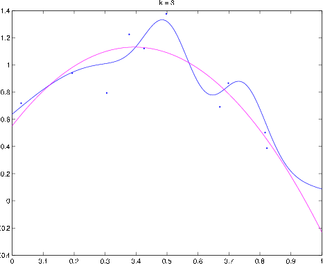
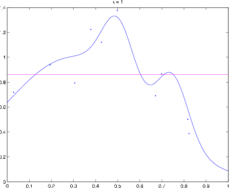
In this case, the classifier which minimizes the empirical risk is
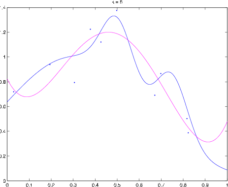
Example polynomial estimator. Blue curve denotes
,
magenta curve is the polynomial fit to the data (denoted by dots).
Overfitting
Suppose
, our collection of candidate functions, is very large. We can always make
smaller by increasing the cardinality of
, thereby providing more possibilities to fit to the data.
Consider this extreme example: Let
be all measurable functions. Then every function
for which
has zero empirical risk (
). However, clearly this
could be a very poor predictor of
for a new input
.
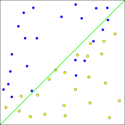
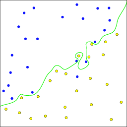
Classification overfitting
Consider the classifier in
[link] ; this demonstrates overfitting in classification. If the data were in fact generated from two Gaussian distributions centered in the upper left and lower right quadrants of the feature space domain, then the optimal estimator would be the linear estimator in
[link] ; the overfitting would result in a higher probability of error for predicting classes of future observations.
Example of overfitting classifier. The classifier's decision boundary wiggles around in order to correctly label the training data, but the optimal Bayes classifier is a straight line.
Regression overfitting
Below is an m-file that simulates the polynomial fitting. Feel free to play around with it to get an idea of the overfitting problem.
% poly fitting
% rob nowak 1/24/04clear
close all
% generate and plot "true" functiont = (0:.001:1)';
f = exp(-5*(t-.3).^2)+.5*exp(-100*(t-.5).^2)+.5*exp(-100*(t-.75).^2);figure(1)
plot(t,f)
% generate n training data & plot
n = 10;sig = 0.1; % std of noise
x = .97*rand(n,1)+.01;y = exp(-5*(x-.3).^2)+.5*exp(-100*(x-.5).^2)+.5*exp(-100*(x-.75).^2)+sig*randn(size(x));
figure(1)clf
plot(t,f)hold on
plot(x,y,'.')
% fit with polynomial of order k (poly degree up to k-1)k=3;
for i=1:k V(:,i) = x.^(i-1);
endp = inv(V'*V)*V'*y;
for i=1:k
Vt(:,i) = t.^(i-1);end
yh = Vt*p;figure(1)
clfplot(t,f)
hold onplot(x,y,'.')
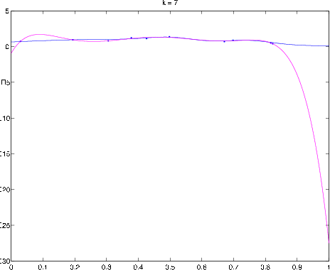
plot(t,yh,'m') Example polynomial fitting problem. Blue curve is
,
magenta curve is the polynomial fit to the data (dots). (a) Fittinga polynomial of degree
: This is an example of underfitting
(b)
(c)
(d)
: This is an example of
overfitting. The empirical loss is zero, but clearly the estimatorwould not do a good job of predicting
when
is close to one.
Questions & Answers
differentiate between demand and supply
giving examples
In economics, a perfect market refers to a theoretical construct where all participants have perfect information, goods are homogenous, there are no barriers to entry or exit, and prices are determined solely by supply and demand. It's an idealized model used for analysis,
When MP₁ becomes negative, TP start to decline.
Extuples Suppose that the short-run production function of certain cut-flower firm is given by: Q=4KL-0.6K2 - 0.112 •
Where is quantity of cut flower produced, I is labour input and K is fixed capital input (K-5). Determine the average product of lab
Kelo
Extuples Suppose that the short-run production function of certain cut-flower firm is given by: Q=4KL-0.6K2 - 0.112 •
Where is quantity of cut flower produced, I is labour input and K is fixed capital input (K-5). Determine the average product of labour (APL) and marginal product of labour (MPL)
Quantity demanded refers to the specific amount of a good or service that consumers are willing and able to purchase at a give price and within a specific time period. Demand, on the other hand, is a broader concept that encompasses the entire relationship between price and quantity demanded
Ezea
ok
Shukri
how do you save a country economic situation when it's falling apart
Economic growth as an increase in the production and consumption of goods and services within an economy.but
Economic development as a broader concept that encompasses not only economic growth but also social & human well being.
Shukri
production function means
Jabir
What do you think is more important to focus on when considering inequality ?
sir...I just want to ask one question... Define the term contract curve? if you are free please help me to find this answer 🙏
Asui
it is a curve that we get after connecting the pareto optimal combinations of two consumers after their mutually beneficial trade offs
Awais
thank you so much 👍 sir
Asui
In economics, the contract curve refers to the set of points in an Edgeworth box diagram where both parties involved in a trade cannot be made better off without making one of them worse off. It represents the Pareto efficient allocations of goods between two individuals or entities, where neither p
Cornelius
In economics, the contract curve refers to the set of points in an Edgeworth box diagram where both parties involved in a trade cannot be made better off without making one of them worse off. It represents the Pareto efficient allocations of goods between two individuals or entities,
Cornelius
Suppose a consumer consuming two commodities X and Y has
The following utility function u=X0.4 Y0.6. If the price of the X and Y are 2 and 3 respectively and income Constraint is birr 50.
A,Calculate quantities of x and y which maximize utility.
B,Calculate value of Lagrange multiplier.
C,Calculate quantities of X and Y consumed with a given price.
D,alculate optimum level of output .
the market for lemon has 10 potential consumers, each having an individual demand curve p=101-10Qi, where p is price in dollar's per cup and Qi is the number of cups demanded per week by the i th consumer.Find the market demand curve using algebra. Draw an individual demand curve and the market dema
suppose the production function is given by ( L, K)=L¼K¾.assuming capital is fixed find APL and MPL. consider the following short run production function:Q=6L²-0.4L³ a) find the value of L that maximizes output b)find the value of L that maximizes marginal product