

| << Chapter < Page | Chapter >> Page > |
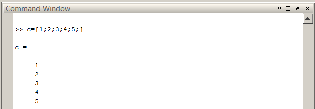
Elements of a column vector is ended by a semicolon:
c = [1;2;3;4;5;]
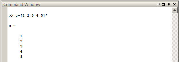
Or by transposing a row vector with the ' operator:
c = [1 2 3 4 5]'
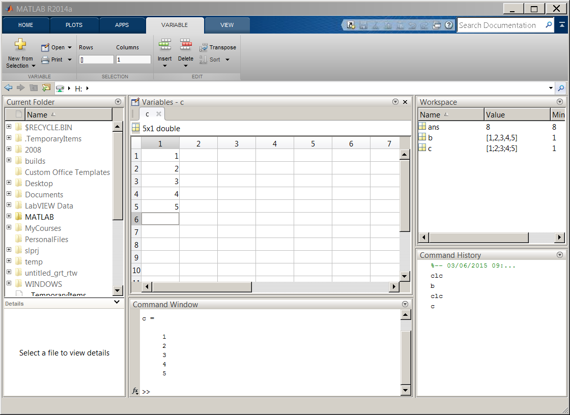
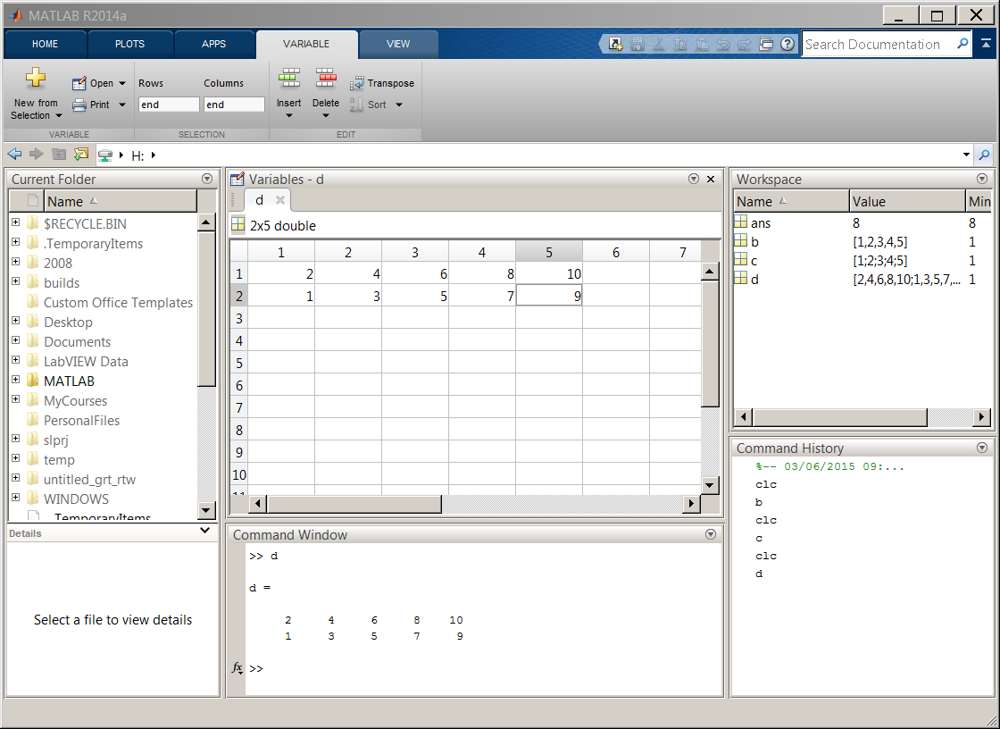
Or by using the Variable Editor:
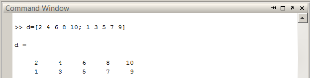
Matrices are typed in rows first and separated by semicolons to create columns. Consider the examples below:
Let us type in a 2x5 matrix:
d = [2 4 6 8 10; 1 3 5 7 9]
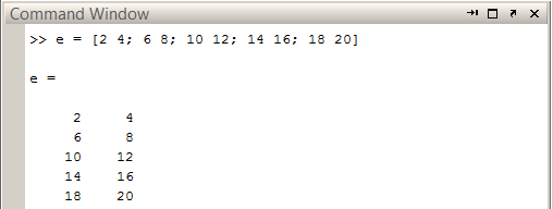
This example is a 5x2 matrix:
Systems of linear equations are very important in engineering studies. In the course of solving a problem, we often reduce the problem to simultaneous equations from which the results are obtained. As you learned earlier, MATLAB stands for Matrix Laboratory and has features to handle matrices. Using the coefficients of simultaneous linear equations, a matrix can be formed to solve a set of simultaneous equations.
Let's solve the following simultaneous equations:
First, we will create a matrix for the left-hand side of the equation using the coefficients, namely 1 and 1 for the first and 2 and -5 for the second. The matrix looks like this:
The above matrix can be entered in the command window by typing
A=[1 1; 2 -5] .
Second, we create a column vector to represent the right-hand side of the equation as follows:
The above column vector can be entered in the command window by typing
B= [1;9] .
To solve the simultaneous equation, we will use the left division operator and issue the following command:
C=A\B . These three steps are illustrated below:
>>A=[1 1; 2 -5]

A =1     1
     2    -5>>B= [1;9]

B =1
     9>>C=A\B

C =2
    -1>>
The result
C indicating 2 and 1 are the values for
x and
y , respectively.
In the preceding section, we briefly learned about how to use MATLAB to solve linear equations. Equally important in engineering problem solving is the application of polynomials. Polynomials are functions that are built by simply adding together (or subtracting) some power functions. (see Wikipedia ).
The coeffcients of a polynominal are entered as a row vector beginning with the highest power and including the ones that are equal to 0.
Create a row vector for the following function:
Notice that in this example we have 5 terms in the function and therefore the row vector will contain 5 elements.
p=[2 3 5 1 10]
Create a row vector for the following function:
In this example, coefficients for the terms involving power of 3 and 1 are 0. The row vector still contains 5 elements as in the previous example but this time we will enter two zeros for the coefficients with power of 3 and 1:
p=[3 0 4 0 -5] .
polyval FunctionWe can evaluate a polynomial
p for a given value of
x using the syntax
polyval(p,x) where p contains the coefficients of polynomial and x is the given number.
Notification Switch
Would you like to follow the 'A brief introduction to engineering computation with matlab' conversation and receive update notifications?

|
|

|
|
|
|
|

|
|

|
|

|
|

|
|

|
|
|
|
|
|
|