

| << Chapter < Page | Chapter >> Page > |
Now we are ready to report the results of the estimation. The key here is to avoid writing a travelog of the estimations. Instead, report all of the regressions in one or more tables and then discuss the results presented in each table.
Since you will find it useful to replicate the estimation of the basic results, this section consists mainly of a set instructions in Table 4 for use with Stata .
| Instruction | Stata commands | |
| 1. | Open Stata and copy the data in Auto_fatalities_data.xls into the data editor. You will have 765 observations of 22 variables. | |
| 2. | Tell Stata what variable denotes the state | .iis |
| 3. | Tell Stata what variable denotes the year | .tis |
| 4. | Create the new variable the percentage of the total vehicle miles driven that are on rural interstate roads | .generate privmd = ruralinterstatevmd/(ruraltotalvmd + urbantotalvmd) |
| 5. | Create the new variable the percent of the total vehicle miles driven that are on urban interstate roads | .generate puivmd= urbaninterstatevmd/(ruraltotalvmd+urbantotalvmd) |
| 6. | Create the logarithm transportation of all of the variables that are not percentages | .generate lz = log(z), where z = dpvmd, sgastax, rsgastax, and rmfi09 |
| 7a. | Estimate the fixed effects model for the linear model (see output in Figure 1) | .xtreg dpvm rsgastax pu25 po70 privmd puivmd rmfi09 bacps, fe vce(robust) vsquish |
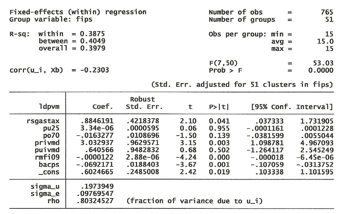
| 7b. | Estimate the fixed effects model for the log-linear model (see output in Figure 2) | .xtreg ldpvm rsgastax pu25 po70 privmd puivmd rmfi09 bacps, fe vce(robust) vsquish |
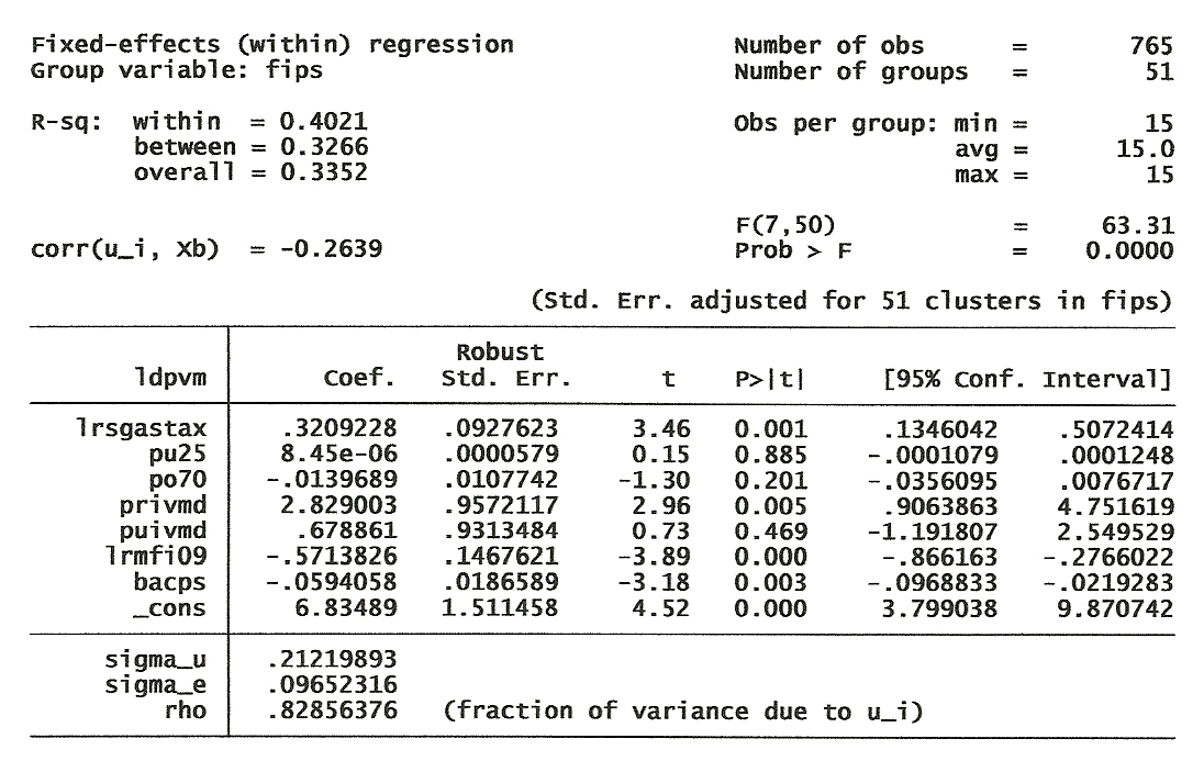
| 7c. | Estimate the fixed effects model for the log-log model (see output in Figure 3) | .xtreg ldpvm lrsgastax pu25 po70 privmd puivmd lrmfi09 bacps, fe vce(robust) vsquish |
| 8. | Place the results into a table making it easier to compare your results; Table 5 is one such table. | |
| 9a. | The results in Table 5 suggest that the per se 0.08 BAC is a successful way to reduce automobile deaths. However the sign on the real gasoline tax rate is the opposite of what we might reasonably expect. Let's check the sensitivity of our results by rerunning the same three regressions with the real gasoline tax replaced by the nominal gasoline tax. See Table 6 for the results of these regressions. | . xtreg dpvm sgastax pu25 po70 privmd puivmd rmfi09 bacps, re vce(robust) vsquish |
| 9b. | .xtreg ldpvm sgastax pu25 po70 privmd puivmd rmfi09 bacps, fe vce(robust) vsquis | |
| 9c. | .xtreg ldpvm lsgastax pu25 po70 privmd puivmd lrmfi09 bacps, fe vce(robust) vsquish |

At this point is makes some sense to compare the parameter estimates for 0.08 BAC per se law; this comparison, shown in Table 5, suggests that the effect of the per se 0.08 BAC law was to reduce fatalities. Moreover, the estimates for each of the models is very stable whether one uses the real price of gasoline or the nominal price of gasoline, thus giving us some more confidence in our conclusions.
| Linear | Log-linear | Log-log | |
| State tax of gasoline in 2009 dollars | |||
| State has a 0.08 per se BAC law | -0.1054 | -0.0692 | -0.0594 |
| (-3.88) | (-3.67) | (-3.18) | |
| State tax of gasoline in current dollars | |||
| State has a 0.08 per se BAC law | -0.1191 | -0.0778 | -0.0762 |
| (-4.83) | (-4.54) | (-4.52) |
The balance of this section of the paper would be devoted to further tests of the stability of our results under varying assumptions. Among other tests one would expect to see if the choice of a fixed-effects model affects your policy conclusions.
This section of your paper should be devoted to a careful recapping of your results and providing suggestions for further research. Such a discussion might include some cautious guesses at why the 0.08 BAC per se standard appears to affect driver behavior. The discussion could also include some estimates of the number of lifes saved by the introduction of a per se standard.
Notification Switch
Would you like to follow the 'Econometrics for honors students' conversation and receive update notifications?

|
|

|
|

|
|

|
|
|
|
|

|
|

|
|

|
|
|
|
|

|