

| << Chapter < Page | Chapter >> Page > |
This method assumes that the inverse transform will produce purely real values in the space domain. Therefore, in the interest of computationalefficiency, the method does not compute the imaginary output values. Therefore, this is not a general purpose 2D complex-to-complex transform. For correct results, the input complex data must match that obtained by performing a forwardtransform on purely real data in the space domain.
Once again it was necessary to sacrifice indentation to force this very long equation to be compatible with this narrow publication format and still bereadable.
| Listing 3. The inverseXform2D method. |
|---|
static void inverseXform2D(double[][]real,
                             double[][] imag,double[][]dataOut){

    int height = real.length;int width = real[0].length;System.out.println("height = " + height);System.out.println("width = " + width);

    //Two outer loops iterate on output data.for(int ySpace = 0;ySpace<height;ySpace++){
      for(int xSpace = 0;xSpace<width;
                                       xSpace++){//Two inner loops iterate on input data.
        for(int yWave = 0;yWave<height;
                                        yWave++){for(int xWave = 0;xWave<width;
                                        xWave++){//Compute real output data.
dataOut[ySpace][xSpace] +=(real[yWave][xWave]*cos(2*PI*((1.0 * xSpace*
 xWave/width) + (1.0*ySpace*yWave/height))) -imag[yWave][xWave]*sin(2*PI*((1.0 * xSpace*
 xWave/width) + (1.0*ySpace*yWave/height))))/sqrt(width*height);
          }//end xWave loop}//end yWave loop
      }//end xSpace loop}//end ySpace loop
}//end inverseXform2D method |
This method requires three parameters. The first two parameters are references to 2D arrays containing the real and imaginary parts of the complexwavenumber spectrum that is to be transformed into a surface in the space domain.
The third parameter is a reference to a 2D array of the same size that will be populated with the transform results.
This method deserves some explanation. The reason that this method is needed is illustrated by Figure 1 .
Both of the images in Figure 1 represent the same wavenumber spectrum, but they are plotted against different coordinate systems.
| Figure 1. Two views of the same wavenumber spectrum. |
|---|
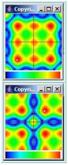 |
The top image shows how the wavenumber spectrum is actually computed.
The wavenumber spectrum is computed covering an area of wavenumber space with the 0,0 origin in the top-left corner. The computation extends to twice theNyquist folding wave number along each axis.
While this format is computationally sound, it isn't what most of us are accustomed to seeing in plots in wavenumber space. Rather, we are accustomed toseeing wavenumber spectra plotted with the 0,0 origin at the center.
Knowing that the area of wavenumber space shown in the top image of Figure 1 covers one complete period of a periodic surface, the shiftOrigin method rearranges the results (for display purposes only) to that shown in the bottom image in Figure 1 . The origin is at the center in the bottom image of Figure 1 . The edges of the lower image in Figure 1 are the Nyquist folding wave numbers.
Notification Switch
Would you like to follow the 'Digital signal processing - dsp' conversation and receive update notifications?

|
|

|
|

|
|

|
|

|
|

|
|

|
|
|
|
|

|
|

|