

| << Chapter < Page | Chapter >> Page > |
| Figure 10. The numeric output for Case A. |
|---|
Case A
Real:1.0 0.923 0.707 0.382 0.0 -0.382 -0.707 -0.923
-1.0 -0.923 -0.707 -0.382 0.0 0.382 0.707 0.923imag:
0.0 0.0 0.0 0.0 0.0 0.0 0.0 0.00.0 0.0 0.0 0.0 0.0 0.0 0.0 0.0 |
If you plot the real and imaginary values in Figure 10 , you will see that they match the transform output shown in graphic form in Figure 9 .
The code from the main method for Case B is shown in Listing 6 . Note that the input complex series contains non-zero values in both the real and imaginaryparts.
| Listing 6. Case B code. |
|---|
System.out.println("\nCase B");
    double[]realInB =
               {0,1,0,0,0,0,0,0,0,0,0,0,0,0,0,1};double[] imagInB ={0,-1,0,0,0,0,0,0,0,0,0,0,0,0,0,-1};

    double[]realOutB = new double[16];double[] imagOutB = new double[16];

    transform.doIt(realInB,imagInB,2.0,realOutB,imagOutB);
display(realOutB,imagOutB); |
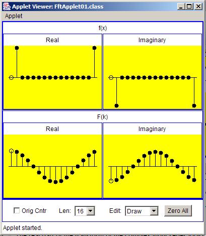
Case B is shown in graphical form in Figure 11 .
| Figure 11. Case B in graphical form. |
|---|
 |
The output from the code in Listing 6 is shown in Figure 12 .
| Figure 12. Case B output in numeric form. |
|---|
Case B
Real:1.0 0.923 0.707 0.382 0.0 -0.382 -0.707 -0.923
-0.999 -0.923 -0.707 -0.382 0.0 0.382 0.707 0.923imag:
-1.0 -0.923 -0.707 -0.382 0.0 0.382 0.707 0.9231.0 0.923 0.707 0.382 0.0 -0.382 -0.707 -0.923 |
If you plot the values for the real and imaginary parts from Figure 12 , you will see that they match the real and imaginary output shown in Figure 11 .
The code extracted from the main method for Case C is shown in Listing 7 .
| Listing 7. Case C code. |
|---|
System.out.println("\nCase C");
    double[]realInC =
      {1.0,0.923,0.707,0.382,0.0,-0.382,-0.707,-0.923,-1.0,-0.923,-0.707,-0.382,0.0,
           0.382,0.707,0.923};double[] imagInC ={0.0,-0.382,-0.707,-0.923,-1.0,-0.923,
           -0.707,-0.382,0.0,0.382,0.707,0.923,1.0,0.923,0.707,0.382};

    double[]realOutC = new double[16];double[] imagOutC = new double[16];

    transform.doIt(realInC,imagInC,16.0,realOutC,imagOutC);
display(realOutC,imagOutC); |
The complex input series for Case C is a little more complicated than that for either of the previous two cases. Note in particular that the input complexseries contains non-zero values in both the real and imaginary parts. In addition, very few of the values in the complex series have a value of zero.
(The values of the complex samples actually describe a cosine curve and a negative sine curve as shown in Figure 13 .)
Case C is shown in graphic form in Figure 13 .
| Figure 13. The graphic form of Case C. |
|---|
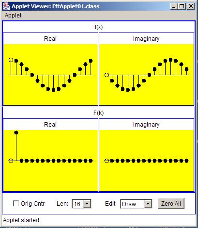 |
The Fourier transform is reversible
One of the interesting things to note about Figure 13 is the similarity of Figure 13 and Figure 5 . These two figures illustrate the reversible nature of the Fourier transform.
If I had used a positive input real value instead of a negative input real value in Figure 5 , the input of Figure 5 would look exactly like the output in Figure 13 , and the output of Figure 5 would look exactly like the input of Figure 13 .
With that as a hint, you should now be able to figure out how I used a mouse and drew the perfect sine and cosine curves in Figure 13 . In fact, I didn't draw them at all. Rather, I used my mouse and drew the output, andthe applet gave me the corresponding input automatically.
Notification Switch
Would you like to follow the 'Digital signal processing - dsp' conversation and receive update notifications?

|
|

|
|

|
|

|
|

|
|

|
|

|
|

|
|
|
|
|

|