

| << Chapter < Page | Chapter >> Page > |
| Original increase in aggregate expenditure from government spending | 100 |
| Which is income to people throughout the economy: Pay 30% in taxes. Save 10% of after-tax income. Spend 10% of income on imports. Second-round increase of… | 70 – 7 – 10 = 53 |
| Which is $53 of income to people through the economy: Pay 30% in taxes. Save 10% of after-tax income. Spend 10% of income on imports. Third-round increase of… | 37.1 – 3.71 – 5.3 = 28.09 |
| Which is $28.09 of income to people through the economy: Pay 30% in taxes. Save 10% of after-tax income. Spend 10% of income on imports. Fourth-round increase of… | 19.663 – 1.96633 – 2.809 = 14.89 |
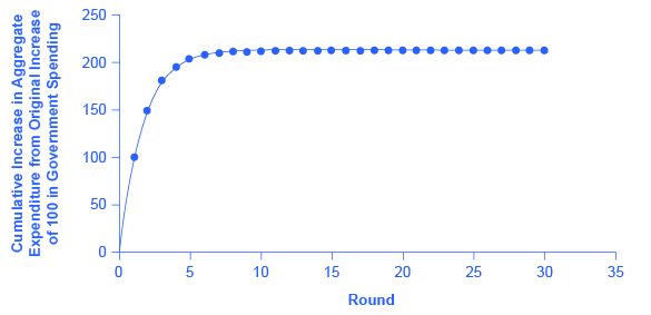
Thus, over the first four rounds of aggregate expenditures, the impact of the original increase in government spending of $100 creates a rise in aggregate expenditures of $100 + $53 + $28.09 + $14.89 = $195.98. [link] shows these total aggregate expenditures after these first four rounds, and then the figure shows the total aggregate expenditures after 30 rounds. The additional boost to aggregate expenditures is shrinking in each round of consumption. After about 10 rounds, the additional increments are very small indeed—nearly invisible to the naked eye. After 30 rounds, the additional increments in each round are so small that they have no practical consequence. After 30 rounds, the cumulative value of the initial boost in aggregate expenditure is approximately $213. Thus, the government spending increase of $100 eventually, after many cycles, produced an increase of $213 in aggregate expenditure and real GDP. In this example, the multiplier is $213/$100 = 2.13.
Fortunately for everyone who is not carrying around a computer with a spreadsheet program to project the impact of an original increase in expenditures over 20, 50, or 100 rounds of spending, there is a formula for calculating the multiplier.
The data from [link] and [link] is:
The MPC is equal to 1 – MPS, or 0.7. Therefore, the spending multiplier is:
A change in spending of $100 multiplied by the spending multiplier of 2.13 is equal to a change in GDP of $213. Not coincidentally, this result is exactly what was calculated in [link] after many rounds of expenditures cycling through the economy.
Notification Switch
Would you like to follow the 'Principles of macroeconomics for ap® courses' conversation and receive update notifications?

|
|
|
|
|

|
|

|
|
|
|
|

|
|

|
|

|
|

|
|

|
|

|
|

|